TL;DR for operators
Cities rarely wait for perfect data. A new district still needs a transit plan, a campus still needs a shuttle model, and a developer still wants to know whether people will walk, drive, or quietly defeat the entire urban-design deck by ordering a car.
The paper behind this article introduces Preference Chain, a method that uses a small sample of behavioural mobility data to guide an LLM agent’s transport choices.1 The important bit is not that it “adds Graph RAG” to an LLM. That phrase now covers everything from serious retrieval systems to someone throwing a Neo4j logo onto a slide. The real mechanism is narrower and more useful: Preference Chain turns sparse human travel records into structured priors over likely choices, then lets the LLM adjust those priors for context.
The result is a useful middle ground. With limited reference data, Preference Chain produces mode and duration distributions closer to Replica mobility data than a raw LLM. It performs especially well when reference data is scarce, around the 50-100 sample range. But once enough labelled data exists, the advantage shrinks; in the paper’s comparisons, an MLP overtakes it as training samples increase. This is not embarrassing. It is the product boundary, which is what mature buyers pay for and immature demos try to hide.
The method also powers a Mobility Agent that simulates 1,000 people moving through Cambridge, MA for 24 hours. Compared with a standard LLM agent, the Mobility Agent improves traffic-flow alignment against Replica data, reducing KLD from 0.814 to 0.621. For POI visits, however, the improvement is tiny: the figure reports 1.718 for the LLM agent and 1.713 for the Mobility Agent. In plain English: Preference Chain helps with travel behaviour more than it solves destination preference.
The business lesson is straightforward. Preference Chain is valuable when an organisation has some behavioural evidence, not enough to train a robust predictive model, and a need to run scenario simulations before better data arrives. It is not a substitute for survey design, local calibration, continuous forecasting, or safety-critical traffic control. It is a cheaper way to stop LLM agents from behaving like generic internet people with fictional commutes. Which, admittedly, is a meaningful improvement.
The planning problem is not “no data”. It is “not enough data yet”.
Urban mobility modelling has a familiar operational problem: the questions arrive before the dataset.
A new neighbourhood is being planned. A transport operator wants to test service coverage. A real-estate team wants to estimate foot traffic. A city wants to evaluate whether a policy change affects workers, students, retirees, and households differently. The serious version of this work uses agent-based models, travel surveys, mobile-device traces, transport counts, POI data, and calibrated choice models. The less serious version asks an LLM what “a typical resident” might do, then pretends the answer is insight. Very efficient. Also very dangerous.
The paper positions Preference Chain between those extremes. Traditional agent-based models can represent populations from the bottom up, but behaviour rules are hard to write and often brittle. Machine-learning and deep-learning models can perform well, but need data volume, feature engineering, and careful calibration. LLM agents can generate plausible choices with little setup, but their plausibility is generic. They know what commuting is. They do not automatically know how commuting behaves in a specific population, city, income band, trip purpose, or time of day.
Preference Chain addresses that gap by asking a different question. Instead of relying on an LLM to invent behaviour from general language priors, can a small set of observed mobility records be organised into a graph that nudges the LLM toward local, population-specific choices?
That is the heart of the paper. Not “LLMs will replace mobility models”. Not “Graph RAG solves transportation”. The contribution is a mechanism for using small behavioural samples as structured decision priors.
Preference Chain is a behavioural prior machine, not a reasoning prompt
The paper contrasts Preference Chain with Chain-of-Thought and Tree-of-Thought prompting. That contrast matters because the method is not trying to make the LLM reason more elaborately. It is trying to make the LLM reason from better behavioural evidence.
A normal prompt might ask:
Given this profile, trip purpose, and time, choose a transportation mode.
The LLM then leans on whatever broad patterns it has absorbed: older people may prefer cars, workers commute in the morning, public transport exists in cities, walking is common for short trips, and so on. Useful, but too generic.
Preference Chain inserts four stages before the final LLM choice:
- Build a behavioural graph.
- Retrieve similar people and relevant behavioural paths.
- Convert graph paths into probabilistic choice priors.
- Ask the LLM to remodel those priors under context.
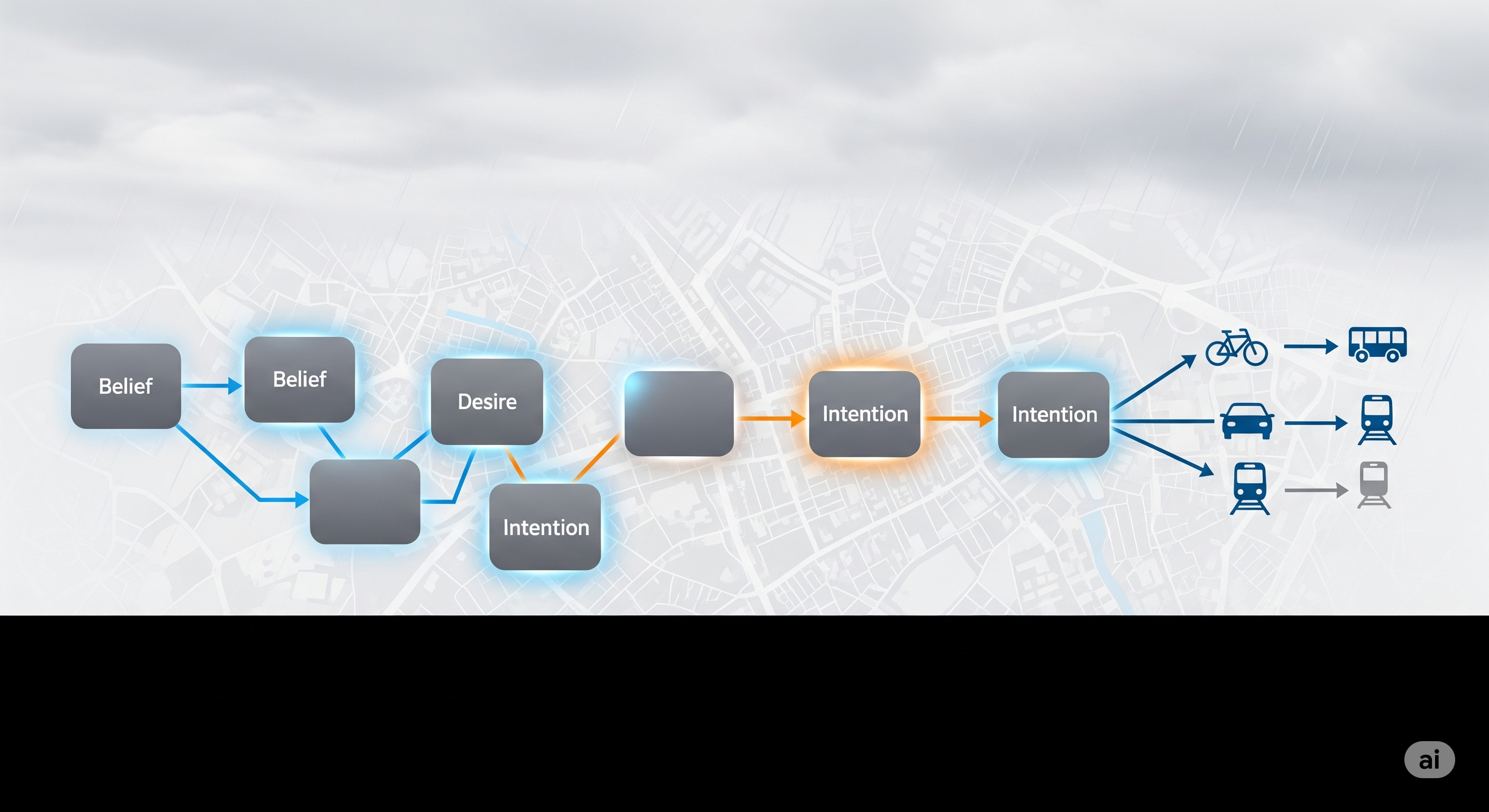
The graph follows a BDI-style structure: Belief, Desire, Intention. In this paper’s mobility setting, the graph contains agents, similar people, desires, and intentions. A desire might represent a travel need, while an intention is the actual candidate behaviour, such as choosing a mode or a duration bin. Edges encode relationships such as profile similarity, desire similarity, social or family closeness, and temporal proximity.
That makes the structure more informative than a simple lookup table. The system is not merely asking, “What did someone like this person do?” It is asking, “What did similar people with similar desires do under related conditions, and how strong are the graph paths connecting this simulated agent to each possible intention?”
The probabilistic step is simple enough to be useful. For each candidate intention, the system searches paths from the agent to that intention. Each path receives a weight based on the product of its edge weights:
The raw score for an intention is the sum of valid path weights:
Those scores are then normalised into a probability distribution over possible choices. The LLM receives these reference choice probabilities and contextual information, then outputs a final set of weighted preferences.
This is why the mechanism-first view matters. Preference Chain is not retrieval as decoration. It is retrieval that produces a usable probabilistic object. The LLM is not the only model. It is the final remodeller of a prior produced by graph search and link prediction.
The LLM’s job is recalibration, not invention
The most interesting design choice is that Preference Chain does not treat the graph output as the final answer. The graph tells the system what happened in similar historical cases. But planning often cares about situations that are adjacent to, not identical with, the reference data.
Weather changes. Trip purpose changes. The city changes. The agent has memory of prior activities. A static probability model can be too literal. A raw LLM can be too imaginative. Preference Chain tries to make the LLM useful by constraining the imagination.
The paper describes the graph probabilities as a prior distribution. The LLM then recalibrates that prior using natural-language context such as time, city, weather, current desire, and agent profile. This is the correct division of labour. The graph supplies local behavioural grounding. The LLM supplies semantic flexibility.
That does not make the LLM magically reliable. It does make the modelling stack less foolish. Instead of asking a language model to generate a commute from vibes, the system asks it to adjust an evidence-derived preference distribution.
There is a practical product pattern here:
| Layer | What it contributes | What can go wrong |
|---|---|---|
| Reference samples | Local or transferable behavioural evidence | Sparse data may miss rare choices |
| BDI graph | Structured links between profiles, desires, and intentions | Edge definitions and weights shape the result |
| Similarity search | Finds comparable people and situations | Similarity may be semantically plausible but behaviourally weak |
| Path-weighted probabilities | Converts retrieved graph structure into choice priors | Frequent behaviours dominate; tails get compressed |
| LLM remodelling | Adjusts priors under contextual conditions | Hallucination, over-smoothing, and discrete-output limits remain |
This is not a data-free model. It is a data-scarce model. That distinction is not pedantry; it is procurement hygiene.
The first experiment tests whether Preference Chain improves a raw LLM
The first experiment is the main evidence for the core method.
The authors use Replica mobility data for Cambridge, MA and San Francisco, CA. The data represent trips on a typical Thursday in Spring 2024 and include traveller attributes such as age, income, employment status, household size, available vehicles, and education level, plus trip purpose, start time, trip duration, and transportation mode. Continuous variables are categorised. The outputs are also discrete: transportation mode and duration bins.
The evaluation compares:
- a raw LLM approach;
- Preference Chain using the same LLM;
- Random Forest;
- XGBoost;
- MLP.
The LLM used for the main experiments is Qwen3:8B without thinking mode. The metrics are Kullback-Leibler Divergence (KLD) for distribution similarity and Mean Average Error (MAE) for prediction accuracy across population groups and choices. Lower is better in both.
The most direct test uses 50 reference samples for Preference Chain and evaluates simulated choices for 1,000 individuals. The result is visually and metrically clear: Preference Chain produces mode and duration distributions closer to the Replica ground truth than the raw LLM. The paper also reports improvement across demographic dimensions.
The interpretation is not “the graph found the truth”. It is narrower: when the LLM is guided by a small behavioural reference set, its generated distribution becomes less generic. The graph pulls it toward observed local choice patterns.
There is also a revealing failure. Preference Chain tends to ignore less frequently chosen options, including on-demand car services, other travel modes, and duration bins longer than 40 minutes. That is exactly the kind of failure one expects from sparse-reference priors. The method learns the central tendency before it learns the tail. For planning teams, that matters. Rare behaviours are not always strategically rare. Airport transfers, late-night trips, disability-access journeys, and emergency-related travel may be low-frequency and high-importance. A model that smooths them away can be operationally neat and strategically wrong. A very tidy way to miss the thing that later appears in the board pack under “unanticipated demand”.
The sample-size curve tells buyers when this is useful
The second part of Experiment I asks how much reference data Preference Chain needs. This is the most commercially relevant result in the paper because it defines the adoption zone.
The paper tests reference sample sizes from 10 to 1,000 and compares Preference Chain with the machine-learning baselines. The core pattern is:
- Preference Chain consistently beats the raw LLM.
- On KLD, Preference Chain performs better than the compared ML methods when reference data is below roughly 100 samples.
- After 100 samples, MLP begins to outperform Preference Chain.
- On MAE, Preference Chain improves up to around 50 samples, then fluctuates without clear further gains.
- MLP gradually surpasses Preference Chain after around 50 samples.
That is a useful boundary, not a weakness. Preference Chain is strongest before conventional supervised learning has enough data to breathe properly. Once the dataset grows, the advantages of trained models reappear.
The paper’s implied sweet spot is therefore not “replace the model”. It is:
Use Preference Chain when the organisation has enough behavioural evidence to anchor an LLM, but not enough labelled data to justify a heavier predictive model.
That zone appears often in practice. Early-stage district planning. New-market mobility studies. Sparse travel surveys. Rural or emerging-city transport analysis. Internal scenario tools before a full digital twin is funded. Pilot deployments where a team needs directional behavioural simulation now and proper model calibration later.
The appendix adds a useful robustness check across LLMs. The authors compare Qwen3:8B, Gemma3:12B, and Llama3.1:8B. Llama3.1 performs better as a baseline without reference data, while Qwen3 performs best once Preference Chain is applied. Across models, gains are strongest when reference data is below about 50 samples, then taper. That supports the mechanism: the improvement is not just one model being lucky. It is a pattern in how sparse reference data improves LLM behavioural simulation.
Still, this is a robustness check, not a second thesis. It suggests model choice matters, but the paper does not establish a universal ranking of LLMs for mobility simulation. The correct takeaway is more modest: Preference Chain’s value appears portable across several open-source LLMs, while absolute performance remains model-dependent.
External-city transfer helps, but local data still wins
The paper then tests a realistic planning problem: what happens when the study area lacks local behavioural data, but another city has usable reference data?
The authors simulate choices in Cambridge using San Francisco reference data, and simulate San Francisco using Cambridge reference data. In both directions, Preference Chain with external reference data improves over the LLM without data. But local data performs better than external data.
This is exactly the result one should hope for. If external data performed as well as local data, the method would look suspiciously insensitive to place. If external data did nothing, it would be less useful for emerging or under-instrumented urban contexts. The observed middle ground is credible: transferable data can improve the LLM, but local calibration still matters.
For operators, this suggests a staged deployment model:
| Stage | Data situation | Sensible use of Preference Chain |
|---|---|---|
| No local data, some comparable-city data | New district, emerging city, early feasibility work | Use external samples for rough behavioural priors |
| Small local sample | Pilot survey, initial trip logs, limited mobility dataset | Build local Preference Chain for scenario testing |
| Growing labelled dataset | More survey waves, sensor data, app logs | Benchmark against supervised ML models |
| Mature data environment | Stable, high-volume labelled data | Use trained models; keep LLM layer only where semantic adaptation is useful |
Preference Chain belongs most naturally in the first two stages. It can also support exploratory analysis in the third. It should not be sold as the final form of a mature forecasting stack unless the buyer enjoys paying premium prices for avoidable underfitting.
The Mobility Agent test shows system value, not just model accuracy
The second experiment embeds Preference Chain inside a broader Mobility Agent. This is where the paper moves from choice modelling to an agent-based urban simulation.
The Mobility Agent has three tools:
- a Profile Generator;
- a Schedule Generator;
- a POI Search Tool.
The simulation creates 1,000 agents in Cambridge for a 24-hour period. Agents receive profiles, generate daily itineraries, use Preference Chain to predict transportation mode and duration, search for nearby POIs based on travel demand and travel constraints, then select destinations. The agent stores important locations such as home, workplace, and school, and keeps memory of information such as date, weather, and prior activities.
This is not merely a larger version of the first experiment. It tests whether the method still helps when individual choices are chained into a spatial simulation. That matters because many agent demos die the moment isolated decisions compound across time and geography. One poor choice is noise. A thousand poor choices become a fake city.
For traffic simulation, the result is promising. Compared with a standard LLM agent, the Mobility Agent aligns better with Replica traffic flow. KLD falls from 0.814 for the LLM agent to 0.621 for the Mobility Agent. The paper also notes that the Mobility Agent identifies Massachusetts Avenue as the primary route, while the LLM agent tends to emphasise Cambridge Street.
The boundary is equally important. Both simulations fail to identify the main traffic corridors along the river because neither accounts for external traffic in Cambridge. That is not a minor footnote. It shows a structural limitation: the agents simulate residents, but not the full traffic system. Commuters, through-traffic, freight, visitors, events, and regional flows can dominate corridors. A resident-agent model can be locally plausible and still miss network-level reality.
For POI visits, the story is weaker. The paper compares simulated POI visits against SafeGraph data. The reported KLD values are nearly identical: 1.718 for the LLM agent and 1.713 for the Mobility Agent. The authors suggest this may be because the reference data lacks direct POI preference information. The Mobility Agent produces a more centralised distribution, probably because travel mode and duration constraints narrow feasible destination choices, but the metric does not show a meaningful POI breakthrough.
That distinction is valuable. Preference Chain improves mobility choices where the reference data contains mobility-relevant behavioural information. It does not automatically infer destination preference if the data does not encode destination preference. Graph RAG is still retrieval. It cannot retrieve what was never represented. Shocking, yes. Also worth remembering.
What each experiment actually supports
The paper contains main evidence, sensitivity testing, transfer testing, system extension, and appendix analysis. Treating all of it as one undifferentiated “results section” would blur the point. Here is the cleaner map:
| Test or figure group | Likely purpose | What it supports | What it does not prove |
|---|---|---|---|
| 50-sample Replica mode/duration simulation | Main evidence | Preference Chain improves raw LLM alignment with observed mode and duration distributions | Full individual-level prediction accuracy or continuous travel-time forecasting |
| KLD/MAE by demographic dimension | Main evidence | Improvements appear across multiple population attributes | Fairness, causal validity, or subgroup reliability under all conditions |
| Reference sample-size comparison | Sensitivity test and comparison with prior work | Preference Chain is strongest under sparse data; MLP overtakes as data increases | That 50-100 samples is universally optimal |
| Cross-city reference data | Robustness / transfer test | External data can improve a raw LLM when local data is missing | That one city can fully substitute for another |
| Different LLMs in appendix | Robustness test | The method’s pattern appears across Qwen, Gemma, and Llama variants | A universal best LLM for mobility agents |
| LLM thinking-output factor analysis | Exploratory diagnostic | The LLM appears to attend heavily to desire and available vehicles, with demographic factors also present | A causal explanation of why the model chooses correctly |
| Mobility Agent traffic simulation | System extension | Preference Chain improves traffic-flow alignment in a 24-hour Cambridge simulation | Full operational traffic forecasting |
| POI visit simulation | System extension with mixed evidence | Travel constraints may shape more plausible POI distributions | Strong destination-choice modelling |
The pattern is coherent. Preference Chain is a strong data-scarce behavioural-choice aid. Its system-level value appears when travel mode and duration influence spatial movement. Its weakness appears when the target behaviour needs information not present in the reference graph.
Business value: cheaper behavioural grounding before expensive calibration
The commercial temptation is to pitch this as “AI agents for transport forecasting”. Resist that. The better pitch is more precise and more credible:
Preference Chain can reduce the cost of early behavioural grounding in agent-based mobility simulations when labelled local data is sparse.
That value lands in several workflows.
First, early-stage planning. Before a city or developer pays for a full study, a Preference Chain-style system could help test whether transport assumptions are obviously fragile across population segments. It will not replace a transport consultant. It might improve the first conversation with one.
Second, scenario exploration. Because the LLM layer can accept natural-language context, planners can test rough changes in time, weather, destination needs, or policy conditions without rewriting a rule base. The graph keeps choices grounded; the LLM keeps the interface flexible.
Third, transfer learning for under-instrumented regions. External reference data is imperfect but useful. For emerging cities, rural areas, informal settlements, or newly developed districts, a method that works better than a raw LLM before local data matures has practical value.
Fourth, digital-twin prototyping. Many digital-twin projects collapse under the weight of data integration before they produce insight. Preference Chain could support lightweight behavioural modules in the prototype phase, especially where the goal is to compare alternatives rather than certify exact forecasts.
Fifth, segmented policy analysis. Because the input features include demographic and socioeconomic variables, the method can simulate heterogeneous population groups. That can help teams ask whether a transport change affects workers, students, lower-income households, older travellers, or carless households differently. It does not prove equity impact, but it can identify where to look.
The ROI logic is not “better than all models”. It is “better than a raw LLM when data is scarce, cheaper than training a mature model before the data exists, and more adaptable than a hand-coded ABM when scenarios are changing.”
That is a narrower claim. It is also the one that might survive procurement.
The misconception: Graph RAG does not abolish data dependency
The likely misreading of this paper is that Graph RAG lets LLM agents behave realistically without data. The paper actually shows the opposite. Preference Chain works because it gives the LLM data, but in a form that is useful under scarcity.
The method needs reference samples. It needs profile variables. It needs choice categories. It needs edge definitions. It needs a graph schema that represents the behaviour being simulated. It benefits from local data. It struggles with rare choices. It does not strongly improve POI visits when POI preference information is missing.
So the better mental model is not:
LLM + Graph RAG = realistic city.
It is:
Sparse behavioural data + graph priors + LLM contextual adjustment = more plausible agent choices under limited evidence.
That replacement matters because it changes implementation priorities. A team adopting this kind of method should not begin by polishing prompts. It should begin by asking what behavioural evidence exists, what choice categories matter, what rare behaviours cannot be lost, and which edge weights deserve domain review.
The graph is not a warehouse for facts. It is a modelling decision surface. Every node type, edge type, weight, and binning choice encodes assumptions. The LLM may make those assumptions feel conversational. It does not make them disappear.
The deployment boundary is sharp enough to be useful
The paper states three key limitations: slow inference, hallucination risk, and discrete modelling. The experiments add several more practical boundaries.
The first boundary is inference speed. LLM-centred simulation is slower than traditional methods. If the system must support real-time traffic control, emergency routing, or high-frequency operational forecasting, this architecture needs serious optimisation and validation before it deserves the room.
The second is tail behaviour. Preference Chain can underrepresent rare options. In mobility, rare does not mean irrelevant. Accessibility trips, on-demand rides, long-duration journeys, and atypical commute patterns may be exactly where policy and commercial risk sits.
The third is data coverage. The method improves what the graph represents. It does not invent reliable POI preference from mode and duration data alone. For destination modelling, operators would need richer reference data about POI choices, land-use attractiveness, opening hours, capacity, pricing, personal preferences, and trip chaining.
The fourth is spatial system completeness. The Cambridge traffic simulation misses river corridors because external traffic is outside the model. A city is not only its residents. It is commuters, visitors, delivery vehicles, service workers, event flows, weather disruptions, and infrastructure constraints. Agent realism at the individual level does not guarantee network realism at the system level.
The fifth is discrete output. The paper categorises variables such as duration into bins. That is sensible for sparse modelling, but unsuitable where continuous estimates are required. A planning dashboard may accept bins. A traffic-control system may not.
The sixth is validation scope. The evidence comes mainly from Cambridge and San Francisco Replica data, plus SafeGraph comparison for POI visits. That is enough to make the method interesting. It is not enough to make it universal.
These limits do not weaken the paper. They make the method legible. Preference Chain is not a final forecasting machine. It is an early-stage behavioural grounding layer for LLM agents.
A sensible implementation playbook
For teams considering a Preference Chain-like architecture, the practical sequence would look something like this:
-
Define the decision target. Mode choice, duration, destination, departure time, route choice, or activity schedule are different behaviours. Do not throw them into one mystical “mobility preference” bucket.
-
Choose the reference sample deliberately. A small local sample may outperform a larger but mismatched external one. If external data is used, document what is transferable and what is not.
-
Design the graph schema with domain experts. Profile similarity, desire similarity, temporal proximity, and choice edges should reflect mobility logic, not just convenient embeddings.
-
Protect rare but important classes. Add minimum-support checks, class-aware weighting, or manual review for categories that sparse data tends to erase.
-
Benchmark against simple baselines. Always compare with raw LLM, simple rules, and conventional ML. If an MLP beats the system once enough data exists, use the MLP. This is not a religion.
-
Separate exploration from operation. Use the LLM layer for scenario design, qualitative adjustment, and prototype simulation. Do not let it silently become an operational control system.
-
Validate at both choice and network levels. A model can predict reasonable mode shares and still create unrealistic traffic corridors. The paper’s Cambridge result makes that point politely; deployment will make it with invoices.
The main managerial implication is that Preference Chain is not a single model purchase. It is a modelling workflow. The asset is the behavioural graph plus the evaluation discipline around it.
The real contribution is disciplined hybridity
The most useful AI systems in specialised domains rarely rely on one capability. They combine structure, data, retrieval, probability, and generation. Preference Chain is a clean example.
The graph alone would be too rigid. The LLM alone would be too generic. A supervised model would need more data. A hand-coded ABM would need more behavioural assumptions. Preference Chain combines the available pieces: sparse behavioural evidence, graph structure, probabilistic priors, and LLM contextual adjustment.
That is the right kind of hybridity. Not glamorous. Not autonomous in the boardroom sense. Not a city planner in a box. Just a method for making synthetic agents a bit less synthetic when local evidence is thin.
For operators, the conclusion is simple: use Preference Chain where the cost of being approximately grounded is lower than the cost of waiting for a mature dataset, and where the decision can tolerate exploratory uncertainty. Do not use it where rare behaviours, continuous forecasts, or safety-critical control dominate the risk profile.
LLM agents do not need to “think like humans” to be useful. They need to stop choosing like untethered autocomplete. Preference Chain gives them a tether. In urban mobility, that is already a meaningful chain of command.
Cognaptus: Automate the Present, Incubate the Future.
-
Kai Hu, Parfait Atchade-Adelomou, Carlo Adornetto, Adrian Mora-Carrero, Luis Alonso-Pastor, Ariel Noyman, Yubo Liu, and Kent Larson, “Graph RAG as Human Choice Model: Building a Data-Driven Mobility Agent with Preference Chain,” arXiv:2508.16172, 2025. https://arxiv.org/abs/2508.16172 ↩︎