Generative models leak. Not because engineers are careless, but because web-scale corpora hide rare, high-influence shards—snippets so unique that gradient descent can’t help but memorize them. A new data-first method, Generative Data Cartography (GenDataCarto), gives teams a way to see those shards in training dynamics and intervene—surgically, not bluntly—before they become liabilities.
The one-slide idea
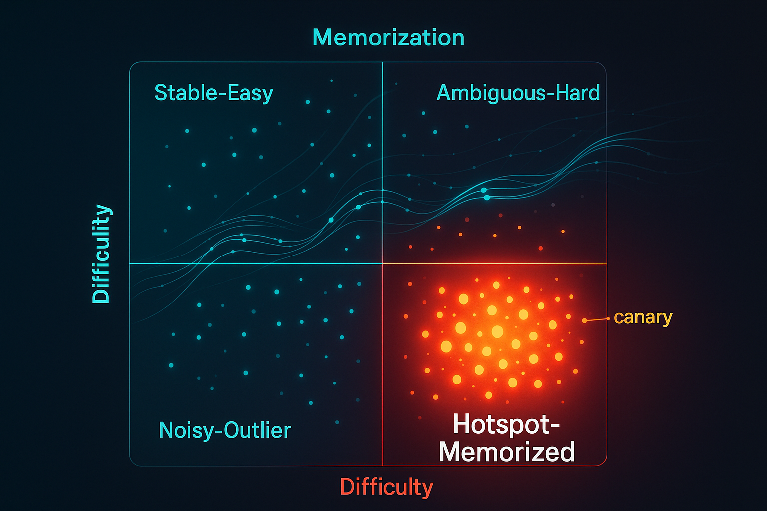
Track two numbers for every pretraining sample:
- Difficulty (dᵢ): early-epoch average loss—how hard it was to learn initially.
- Memorization (mᵢ): fraction of epochs with forget events (loss falls below a threshold, then pops back above)—how often the model “refits” the same sample.
Plot (dᵢ, mᵢ), set percentile thresholds, and you get a four-quadrant map that tells you what to up-sample, down-weight, or drop to reduce leakage with minimal perplexity cost.
The quadrant map (use this in your data room)
| Quadrant | Rule | Interpretation | Default Intervention |
|---|---|---|---|
| Stable–Easy | dᵢ ≤ τ_d, mᵢ ≤ τ_m | Core, well-learned patterns | Keep or lightly up-sample |
| Ambiguous–Hard | dᵢ > τ_d, mᵢ ≤ τ_m | Challenging but not memorized | Up-sample (γ>1) to improve robustness |
| Hotspot–Memorized | dᵢ ≤ τ_d, mᵢ > τ_m | Easy yet repeatedly re-fit → high extraction risk | Down-weight (α<1) or prune |
| Noisy–Outlier | dᵢ > τ_d, mᵢ > τ_m | Hard and memorized → likely corrupted/odd | Remove if quality is suspect |
Why it works: Under standard smoothness/stability assumptions, mᵢ is a lower bound proxy for per-sample influence. Down-weighting high‑mᵢ points provably tightens the generalization gap; empirically it cuts canary extraction by 30–60% with ~0–1% perplexity hit.
How to implement in a real pretraining run
-
Record per-sample losses by epoch (or steps) for a burn‑in window (Tₑ). Store an epoch×sample matrix L.
-
Compute scores
- Difficulty: dᵢ = mean(L₁:ₜₑ,ᵢ)
- Memorization: mᵢ = share of transitions where Lₜ,ᵢ < ε and Lₜ₊₁,ᵢ > ε
-
Choose thresholds (e.g., τ_d=75th percentile of dᵢ; τ_m=25–35th of mᵢ depending on risk appetite).
-
Reweight your sampler after burn‑in: up-sample Ambiguous–Hard, down‑weight or drop Hotspot–Memorized/Noisy‑Outliers.
-
Lock a governance loop: track canary recall, MI‑AUC (membership inference), and held‑out perplexity per intervention level; pick the knee of the curve.
What this changes for data and risk leaders
- From model-only to data-first safety. You don’t need DP-SGD or heavyweight filters to get meaningful leakage reductions. Start by curating gradients with reweighting.
- Quantified trade-offs. Down‑weighting ∆α of N_hot hotspot samples reduces expected generalization gap by ≥ 2β∆αN_hot (β: stability). In practice, that’s security gain without throwing away benchmark performance.
- Auditable datasets. The (dᵢ, mᵢ) map surfaces “why is this here?” content—PII, copyrighted passages, benchmarks—earlier in the pipeline, enabling targeted removals and documentation.
Where to deploy first (concrete playbook)
- Pre‑release red team: run GenDataCarto on your last pretraining checkpoint; prune top‑mᵢ tail (5–10%). Measure canary extraction and MI‑AUC before/after.
- Benchmark hygiene: flag any evaluation samples that appear in Hotspot–Memorized; replace or mask to avoid contamination bias.
- Vendor ingestion: require third‑party corpus providers to ship (dᵢ, mᵢ) summaries; reject batches with excessive hotspot mass.
- Regulated domains: for legal/health data, set a stricter τ_m (e.g., 20th percentile) and apply automatic down‑weighting rather than hard drops to preserve distribution shape.
Practical knobs (and sensible defaults)
- Burn‑in Tₑ: 10–20% of total epochs—enough to stabilize early loss but before heavy overfitting.
- Forget threshold ε: relative (e.g., min‑loss + δ) to adapt across samples; sweep δ for stability.
- Reweighting: start with α=0.5 for hotspots; γ=1.5–2.0 for ambiguous‑hard.
- Monitoring: track extraction success vs. pruned weight and ∆perplexity vs. pruned weight; choose the Pareto knee.
Limitations (read before rolling to prod)
- Logging cost: you need per-sample loss logging; use micro‑batch hooks and periodic sampling to cap IO.
- Assumption gaps: proofs use convex/smooth surrogates; results are empirical for deep nets—treat as signals, not absolutes.
- Distribution shift risk: aggressive pruning can distort long‑tail semantics; prefer down‑weighting to deletions unless content is clearly toxic/private.
The Cognaptus take
Data cartography is the missing safety dashboard for foundation models. It doesn’t replace DP, red‑teaming, or post‑hoc filters; it prioritizes them by showing where your gradient budget is most dangerously concentrated. If you’re training or fine‑tuning this quarter, wire up per‑sample losses, draw the map, and put risk controls on the hotspots. It’s cheap, measurable, and it moves the leakage needle.
—
Cognaptus: Automate the Present, Incubate the Future