TL;DR for operators
Models rarely fail because nobody ran a sensitivity analysis. They fail because the sensitivity analysis answered the convenient question instead of the relevant one.
The paper behind gsaot introduces an R package for Optimal Transport-based global sensitivity analysis.1 Its practical value is not that it makes Sobol’ indices obsolete. It does not. The useful shift is narrower and more interesting: gsaot estimates how much the entire output distribution changes when an input is known, rather than asking only how much of the output variance can be attributed to that input.
That matters when the output is not a single scalar. A climate trajectory, a dynamic ecological system, a multivariate risk vector, or a simulation path is not well served by pretending that one summary statistic has captured the business question. That little act of compression is where many elegant dashboards quietly become decorative furniture.
The package is designed for given-data estimation. In plain terms, if you already have a dataset of model inputs and outputs, gsaot can post-process it. The model can be written in R, Python, C++, Excel held together by prayer, or retrieved from an existing experiment. The package does not need to own the simulation pipeline.
The paper’s contribution is therefore mostly operational. It packages recent Optimal Transport sensitivity indices into usable R workflows: classical and entropic OT solvers, one-dimensional shortcuts, Wasserstein-Bures decomposition, bootstrap intervals, local separation plots, solver comparison, custom costs, and dummy-variable thresholds for numerical noise.
For business use, the main opportunity is cheaper diagnosis: rank the drivers of complex models, find parameters worth fixing, decide where to refine scenarios, and document why certain uncertainties matter. The main caveat is equally practical: these indices are only as credible as the sample size, partitioning, solver configuration, regularisation level, and output distance metric used to compute them.
The old question was variance; the new question is movement
Sensitivity analysis usually begins with a management-friendly question: which inputs matter?
That question sounds simple until the output stops being simple. A single profit number, default probability, crop yield, or engineering tolerance can be handled with familiar variance-based machinery. But many modern models produce objects: vectors, spatial fields, time series, correlated risk measures, policy trajectories. Once the output is a shape rather than a number, “which input explains the variance?” becomes less a scientific question and more a request to choose which detail to ignore.
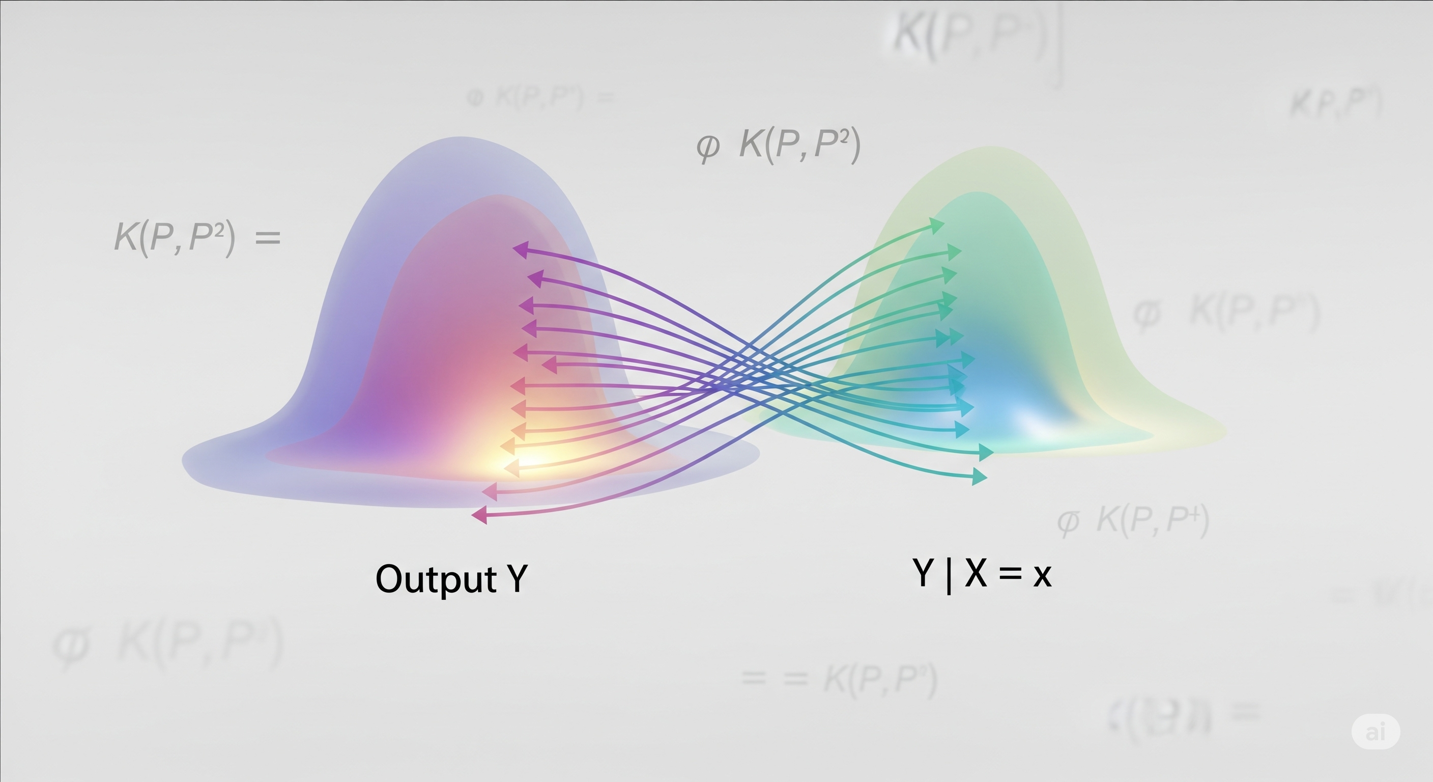
The mechanism in this paper starts from a more general view. Take the model output distribution. Then condition on one input. If knowing that input changes the output distribution a lot, the input is important. If the conditional output distribution looks almost like the unconditional one, the input is not doing much.
That is the central move:
The package uses Optimal Transport as the separation measure. Instead of comparing two distributions only by mean or variance, OT asks how much “work” is required to move one distribution into the other. This is why the article’s title gets away with invoking Sinkhorn without committing a felony against nuance.
The paper’s theoretical setup defines a local separation for each input value and then averages it into a global index. The local part is important. It means the analyst can ask not only “does this input matter?” but also “where in its range does it matter?” A parameter may be harmless in the middle and dangerous at the edges. Anyone who has ever managed a real portfolio, supply chain, or climate scenario knows this is usually where the bodies are buried.
What gsaot actually contributes
The paper is not claiming to invent Optimal Transport sensitivity analysis from scratch. It operationalises recent OT-based sensitivity measures in an R package and wraps them in a workflow analysts can actually run without hand-assembling solvers, estimators, plots, and diagnostic checks.
That distinction matters. Research methods often die in the swamp between theorem and spreadsheet. gsaot is a bridge across part of that swamp.
| Technical contribution | Operational consequence | ROI relevance |
|---|---|---|
| Given-data estimation | Works from an existing input-output dataset rather than requiring a special simulation design | Reuses expensive simulation runs and historical experiment outputs |
| Correlated-input support | Does not require the artificial independence assumptions common in simpler workflows | More realistic risk, climate, engineering, and socio-economic modelling |
| Multivariate and time-dependent outputs | Treats output curves or vectors as the object of analysis | Avoids collapsing trajectories into one convenient but lossy statistic |
| Classical OT solvers | Supports exact OT computation through established transport algorithms | Useful when precision matters and compute is acceptable |
| Entropic Sinkhorn solvers | Provides faster approximate computation through regularised OT | Useful for larger workflows, provided regularisation is interpreted correctly |
| Wasserstein-Bures decomposition | Splits influence into mean-related and covariance-related components under suitable conditions | Helps explain whether an input shifts levels, volatility, correlation, or both |
| Bootstrap intervals | Adds uncertainty estimates around indices | Helps separate stable rankings from numerical theatre |
| Dummy-variable thresholds | Estimates the level of numerical noise from an irrelevant synthetic input | Helps decide when a small non-zero index should be ignored |
The package includes several solver pathways. For one-dimensional outputs, it can exploit quantile-based OT computation. For Gaussian or suitable elliptical settings with squared Euclidean costs, it can use the Wasserstein-Bures form, which decomposes the transport cost into mean and covariance components. For general multivariate outputs, it can call classical transport solvers or entropic Sinkhorn variants.
This is not just a menu of options. It is a set of trade-offs. One-dimensional shortcuts are fast but narrow. Wasserstein-Bures decomposition is interpretable but depends on distributional structure. Classical OT is more faithful but computationally heavier. Sinkhorn is faster, but regularisation changes the object being estimated.
The package does not abolish judgement. It relocates judgement to places where analysts can see it.
Sinkhorn is not magic; it is a regularised bargain
A likely misreading of the paper is that Sinkhorn simply makes OT sensitivity analysis faster. That is true, in the same way that a credit card makes things affordable. The bill still arrives.
Classical Optimal Transport has attractive theoretical properties. The OT-based sensitivity index is normalised between zero and one, reaches zero under independence, and reaches one under a deterministic functional relationship between input and output. These properties are valuable because they make the index interpretable as a statistical association measure, not just as an arbitrary score.
Entropic regularisation changes the computation. It adds a penalty term that makes the optimisation problem easier to solve and allows the fast Sinkhorn-Knopp algorithm. As the regularisation parameter $\epsilon$ tends toward zero, the entropic solution approaches the classical OT solution under broad conditions. That is the useful part.
But the entropic index does not preserve strict zero-independence in the same clean way. Even under independence, the lower bound is positive. The paper is explicit on this point: entropic OT indices can be used as meaningful sensitivity measures in their own right, or as fast approximations to classical OT for small $\epsilon$. Those are not the same claim.
This distinction is not academic hair-splitting. If a modeller uses a large $\epsilon$, the ranking may still look right while the values become inflated. In the paper’s Gaussian example, large regularisation correctly identifies the importance ranking, but the entropic indices are more than 0.25 higher on average than the classical and Wasserstein-Bures alternatives. Small regularisation produces values comparable to the other methods.
That is a nice result because it is not too nice. It says Sinkhorn can be useful, but only if the user remembers that speed is not a sacrament.
The Gaussian example validates the machinery, not the universe
The first example uses a bivariate linear Gaussian model with three correlated inputs. This is the clean-room test. The analytical OT-based indices are known: $X_2$ and $X_1$ dominate, with total indices around 0.507 and 0.492 respectively, while $X_3$ sits much lower at 0.117. The decomposition shows that $X_1$ and $X_2$ affect both the mean and covariance of the bivariate output.
This example is mainly main evidence for implementation correctness. The authors use it to check whether gsaot reproduces known analytical values and to demonstrate core functions.
The package estimates Wasserstein-Bures indices close to the analytical values with $N = 2000$ simulations and $M = 20$ partitions. The printed result gives total indices of roughly 0.470 for $X_1$, 0.499 for $X_2$, and 0.117 for $X_3$. With bootstrap enabled, the package reports 95% confidence intervals, such as approximately 0.452 to 0.479 for $X_1$, 0.482 to 0.508 for $X_2$, and 0.096 to 0.123 for $X_3$.
The business interpretation is modest but useful. This is not evidence that every real model will behave politely. It is evidence that the implementation can recover the expected structure in a case where the truth is known.
The solver comparison in the same example is best read as a solver sensitivity test. Wasserstein-Bures and classical network-flow OT estimates are close to the analytical solution. Sinkhorn with small $\epsilon$ is also close. Sinkhorn with large $\epsilon$ preserves the ranking but inflates the scores. This is exactly the kind of result operators should want: not a sales pitch, but a warning label with numbers attached.
| Test in the paper | Likely purpose | What it supports | What it does not prove |
|---|---|---|---|
| Linear Gaussian model with analytical indices | Main implementation validation | gsaot can recover known rankings and approximate known values | Performance on arbitrary nonlinear models |
| Wasserstein-Bures decomposition | Interpretability demonstration | Inputs can be separated into mean and covariance effects under suitable assumptions | That all output differences are captured by first two moments |
| Solver comparison | Solver sensitivity test | Small-$\epsilon$ Sinkhorn can approximate classical OT; large $\epsilon$ can inflate scores | That Sinkhorn is universally safe or automatically calibrated |
| Bootstrap intervals | Estimation uncertainty demonstration | Rankings can be shown with uncertainty bands | That bootstrap alone resolves model-design uncertainty |
The example also demonstrates ot_indices_smap, which computes one-dimensional sensitivity maps for each output component. In the paper, $X_1$ has stronger impact on $Y_1$, while $X_2$ dominates $Y_2$. This is a small but important workflow point: multivariate sensitivity is useful, but sometimes management still needs to know which component of the output is being moved.
The budworm model shows why trajectories need distributional sensitivity
The second example moves from clean validation to a dynamic ecological model: the spruce budworm and forest system. The model has ten inputs and three time-dependent outputs: budworm density, average tree size, and tree energy reserve. The authors run $N = 2000$ simulations and treat each output trajectory as a multivariate object.
This example is main evidence for time-dependent output handling, with a side role as a comparison with prior work because the authors compare its conclusions to earlier analysis by Puy and colleagues.
The important result is not only which inputs rank highest. It is that gsaot can rank inputs for whole trajectories without forcing the analyst to reduce each trajectory to a single endpoint, peak, average, or other analyst-chosen summary. That is a material advantage. In dynamic systems, the moment of divergence is often as important as the final value.
For output $B$, the budworm density, the printed indices identify $K$ as dominant at about 0.583 and $r_S$ as second at about 0.215. Most other inputs hover near small non-zero values. This creates a common interpretive problem: are those small values real, or just numerical noise wearing a lab coat?
The paper handles this with a dummy-variable irrelevance threshold. The package generates an input independent of the output. In theory, its OT-based index should be zero. In practice, any non-zero estimate gives a sense of numerical noise. Inputs close to that dummy threshold can be treated as potentially irrelevant.
This is one of the most operationally valuable parts of the paper. Business users rarely need a theological debate over whether a score of 0.026 is “real”. They need a disciplined way to decide whether to spend modelling budget on it.
The budworm results show:
| Output trajectory | Inputs identified as important | Interpretation |
|---|---|---|
| Budworm density $B$ | $K$ and $r_S$; possibly small contribution from $T_E$ | Density is mainly shaped by carrying-capacity and growth dynamics |
| Average tree size $S$ | $r_S$ and $K$; possibly small contribution from $T_E$ | Tree-size trajectory depends heavily on branch growth and carrying structure |
| Energy reserve $E$ | $K_E$, $K$, $\alpha$, and $T_E$ | Energy dynamics have a different sensitivity profile than density or size |
The local separation plots add another layer. For output $B$, the effect of $K$ and $r_S$ is strongest at extreme values, especially low values, while central regions have much smaller impact. That is not a trivial detail. A global ranking tells the operator what matters on average; local separation tells the operator where stress-testing should concentrate.
If you manage scenario analysis, that is the difference between “watch parameter K” and “watch the low-end region of K, because that is where output behaviour actually changes.” One is a dashboard note. The other is an operating instruction.
The climate example makes the distance metric part of the business question
The third example uses a simplified climate module inspired by DICE2016. The model produces atmospheric temperature anomaly trajectories, and the authors compute OT-based indices with a custom ground cost: a Minkowski distance of order 3, cubed. They use Sinkhorn with $\epsilon = 0.001$, bootstrap intervals with 100 replicates, and an irrelevance threshold.
This example is best read as an implementation detail plus exploratory extension. Its purpose is to show that gsaot can handle custom costs for structured outputs, not to establish a new result about climate policy.
The distinction is important. The climate model result identifies $\phi_{11}$ as the leading driver, with an index around 0.212 in the printed output and 0.218 in the bootstrap table. Climate sensitivity $S$ follows at about 0.079 to 0.085. Parameters $c_1$ and $\lambda$ are above the dummy threshold but much smaller. The dummy threshold is about 0.0265, which puts several small indices in the numerical-noise neighbourhood.
The paper concludes that $\phi_{11}$, $S$, $c_1$, and $\lambda$ are relevant, while variables such as $\phi_{23}$, $c_3$, $c_4$, $F_{EX0}$, and $F_{EX1}$ are small. Local separation plots for low-ranked inputs show small effects across their domains, supporting the practical decision to fix those inputs in future analyses.
The deeper business lesson is about the cost function. When outputs are trajectories, “distance” is not neutral. A cost metric encodes what kinds of differences matter. Does the analyst care about late-century deviation, short-term overshoot, shape, peak timing, cumulative exposure, or smoothness? gsaot permits custom ground costs, which is powerful precisely because it makes that modelling judgement explicit.
That power comes with responsibility, unfortunately. A custom distance metric can align sensitivity analysis with the business question. It can also smuggle in a preference structure nobody has reviewed. The package gives the knife; governance must decide whether anyone is allowed to juggle it.
The business value is cheaper diagnosis, not prettier maths
For a company using simulation models, the direct value of gsaot is not “better AI” or “more advanced analytics”. It is model triage.
A practical workflow might look like this:
- Run or collect a Monte Carlo input-output dataset from the existing model.
- Choose an output representation: scalar, vector, time series, or structured trajectory.
- Select a cost metric that matches the operational question.
- Estimate OT-based indices with appropriate solvers.
- Compare solver choices where feasible.
- Use bootstrap intervals and dummy-variable thresholds to separate robust drivers from numerical residue.
- Use local separations to identify where important inputs matter.
- Fix or deprioritise low-impact inputs in future runs, scenarios, or reporting.
The result is not just a ranking. It is a way to reduce modelling clutter.
For risk engines, this can identify which assumptions actually move portfolio loss distributions rather than just average loss. For climate or energy models, it can separate parameters that shape whole trajectories from parameters that only make tiny local adjustments. For engineering simulations, it can help focus calibration on variables that move multivariate performance envelopes. For economic and policy models, it can support scenario prioritisation without pretending that correlated inputs live in splendid isolation.
This is where the given-data design matters. Many organisations already have expensive simulation archives. They do not want to rerun a model under a sampling design invented after the budget was spent. gsaot’s post-processing orientation makes it compatible with that institutional reality.
No, this does not remove the need for careful experimental design. But it does make sensitivity analysis less dependent on having planned everything perfectly before the first simulation run. In business, that counts as mercy.
Where the paper’s evidence is strongest
The paper is strongest as a package and workflow paper. It gives theory, implementation, and examples. It does not pretend to be a benchmarking paper across every sensitivity-analysis library under every data regime.
The evidence base is coherent:
| Evidence component | Role in the paper | Strongest support |
|---|---|---|
| Theory section | Mechanism and index properties | Why OT-based indices can capture distributional dependence and support multivariate outputs |
| Solver implementation | Computational bridge | How classical and entropic OT become practical in R workflows |
| Gaussian example | Validation | Estimates align with analytical values and show solver/regularisation behaviour |
| Budworm model | Dynamic-output demonstration | Whole trajectories can be analysed, with dummy thresholds and local separations |
| Climate model | Custom-cost demonstration | Analysts can adapt the output distance metric to the structure of the problem |
The Gaussian example is the most controlled. The budworm example is the most persuasive for dynamic modelling. The climate example is the most relevant to business governance because it exposes the role of the cost metric.
This matters because a bad reading of the paper would ask, “Does gsaot beat Sobol’?” That is not quite the point. Sobol’ indices answer a variance-decomposition question under assumptions and designs that are often useful. gsaot answers a broader distributional-dependence question under a given-data estimation workflow. The better question is: when is variance not enough?
Boundaries operators should not ignore
The paper is useful because it is concrete. The boundaries are concrete too.
First, the number of partitions matters. Given-data estimation approximates conditioning by partitioning the input support. Too few partitions blur local behaviour. Too many partitions leave too little data per partition. The authors discuss this directly and suggest ensuring at least 100 points per partition for sample sizes between 100 and 10,000. At larger sample sizes, previous work suggests a plateau effect where estimates become less sensitive to partition choice.
Second, numerical noise is not optional decoration. Small non-zero OT indices can appear even for irrelevant variables. The dummy-variable threshold is therefore not a cute feature; it is a necessary sanity check, especially in small or computationally difficult settings.
Third, Sinkhorn regularisation must be tuned and interpreted. Large $\epsilon$ can preserve ranking but inflate values. Small $\epsilon$ can approximate classical OT better but may increase computational burden or numerical difficulty. The paper demonstrates both sides.
Fourth, the cost function defines what “different outputs” means. For scalar output, that may be straightforward. For time series, spatial fields, or multivariate risk vectors, it is a modelling decision. A bad metric can produce a formally correct answer to the wrong operational question. Very efficient nonsense remains nonsense, just with better runtime.
Fifth, Wasserstein-Bures decomposition is interpretable but not universal. It cleanly separates mean and covariance effects under appropriate distributional conditions, such as Gaussian or related elliptical settings. Outside those conditions, higher-order distributional differences may matter, and the decomposition should not be oversold.
Finally, gsaot is a package for sensitivity analysis, not a substitute for domain modelling. It can reveal which inputs move outputs in the dataset provided. It cannot guarantee that the dataset spans the right domain, that the simulator is valid, or that the organisation asked the right policy question. Software rarely fixes epistemology. It mostly makes epistemology faster.
The practical upgrade is distributional accountability
The real contribution of gsaot is not that it replaces familiar sensitivity tools. It gives analysts a usable route into a broader diagnostic regime: correlated inputs, multivariate outputs, given-data estimation, solver flexibility, uncertainty intervals, local effects, and noise thresholds.
That is a meaningful upgrade because many models now produce outputs that are richer than the methods used to interrogate them. A firm may simulate thousands of climate paths, portfolio loss surfaces, demand trajectories, or system states, then collapse them into a single summary because the sensitivity method expects a scalar. At that point, the analysis has already negotiated away part of the problem.
Optimal Transport-based sensitivity analysis offers another option. It asks how the output distribution moves when an input is known. gsaot makes that question easier to ask in R.
The paper’s lesson for operators is simple enough: use Sobol’ when the variance question is the right question. Use distributional transport when the output object is richer, the inputs are correlated, and the cost of ignoring shape is higher than the cost of computation.
Not every model needs this. But the models that do need it are usually the ones sitting closest to expensive decisions. Naturally.
Cognaptus: Automate the Present, Incubate the Future.
-
Leonardo Chiani, Emanuele Borgonovo, Elmar Plischke, and Massimo Tavoni, “gsaot: an R package for Optimal Transport-based sensitivity analysis,” arXiv:2507.18588, 2025. https://arxiv.org/pdf/2507.18588 ↩︎