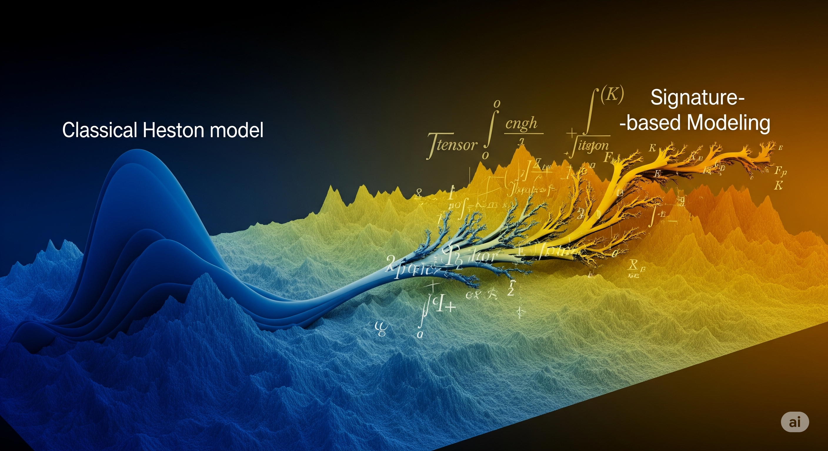
Financial engineers have long sought to tame the volatility surface. From Black-Scholes to Heston, modelers have used parametric tricks to approximate implied volatilities across strikes and maturities. But what happens when the surface refuses to play along—when volatility is rough, the market isn’t Heston, and no closed-form expansion suffices?
In today’s article, we explore a signature-based approach from rough path theory that aims to solve this exact problem. The method not only matches the performance of classical asymptotic expansions in well-behaved markets, but even excels when things get bumpy.
From Classical Expansions to Signature Flexibility
The benchmark method in this space is the second-order asymptotic expansion by Alòs et al. (2015), which assumes the asset follows Heston dynamics:
\begin{align*} dS_t &= r S_t dt + \sigma_t S_t d(\rho W_t + \sqrt{1 - \rho^2} B_t) \ d\sigma^2_t &= \kappa(\theta - \sigma^2_t) dt + \nu \sqrt{\sigma^2_t} dW_t \end{align*}
Using Malliavin calculus, Alòs and coauthors derive explicit approximations of implied volatility as functions of maturity $T$, log-moneyness $x - k$, and Heston parameters $\theta, \nu, \kappa, \rho, \sigma_0$. The result: a fast, elegant calibration method when the model holds.
But if the market strays from Heston-like behavior—say, into rough volatility territory—this expansion loses accuracy.
That’s where signatures come in.
A Signature Move: Modeling Volatility with Iterated Integrals
Rough path theory replaces rigid model assumptions with function approximation. Instead of assuming a particular SDE, we represent the volatility $\sigma_t$ as a linear functional of the signature of a primary process $X$:
$$ \sigma_t(\ell) = \langle \ell, S(X)^{\leq N}_t \rangle $$
Here, $S(X)^{\leq N}_t$ is the truncated signature of the path $X$ up to level $N$. It encodes iterated integrals of $X$, including quantities like:
- $\int_0^t X_s dX_s$ (second-order)
- $\int_0^t \int_0^s X_u dX_u ds$ (third-order)
These terms collectively capture the shape of the path in a way that’s universal: any continuous functional of the path (like volatility) can be approximated linearly in signature space. That’s the magic.
A key advantage? You’re no longer assuming that the market follows Heston, SABR, or any parametric model. You just learn the shape.
Head-to-Head: Signature vs. Asymptotic Expansion
The authors calibrate both methods on synthetic markets with known ground truth:
1. Heston Market ($\rho = 0$ and $\rho = -0.5$)
- Result: Signature calibration matches asymptotic expansion accuracy to within $10^{-3}$ in implied volatility.
- Observation: Signature learns the correct coefficients $\ell$ even when initialized with different volatility dynamics.
- Computation: Full-surface calibration with signature (N=3, 15 terms) completes in ~90 minutes on standard hardware; local smiles take ~4 minutes.
2. Rough Bergomi Market ($H = 0.1$)
- Result: Signature method fits implied vol surface better than the asymptotic method, which breaks down due to model mis-specification.
- Insight: Even with a primary process that’s not rough (e.g. Heston), the signature model adapts.
| Market Model | Calibration Method | Max Error (IV) | Flexibility | Assumes Parametric Form? |
|---|---|---|---|---|
| Heston | Asymptotic (Alòs et al.) | ~0.001 | Low | Yes |
| Heston | Signature-Based | ~0.001 | High | No |
| Rough Bergomi | Asymptotic | High (fails) | None | Yes |
| Rough Bergomi | Signature-Based | ~0.001 | High | No |
The Cost of Generality
The catch? Computing signature terms—especially for pricing formulas involving terms like $Q(t)_{ij} = \langle (e_I \shuffle e_J) \otimes e_0, S(X)_t^{\leq 2N+1} \rangle$—requires high-dimensional tensor algebra.
The signature vector grows exponentially with truncation level:
$$ \text{dim}(S^{\leq N}) = 2^{N+1} - 1 $$
At $N = 3$, the vector has 15 terms. But to compute certain pricing terms, you may need access to 255 signature coordinates (level 7). This isn’t prohibitive, but it does demand GPU acceleration and care.
Still, thanks to factorial decay, higher-order signature terms become negligible quickly. This keeps the optimization problem well-behaved.
What This Means for Practitioners
- Speed vs. Flexibility: If you know the market follows Heston, asymptotic expansions remain unbeatable for speed.
- When in Doubt, Signatures Win: If you’re unsure about market structure—or if roughness, skew, or nonlinearity dominate—signature-based calibration is your friend.
- No Need for PDEs or Greeks: Signatures let you learn volatility dynamics from paths directly, sidestepping PDE solvers and manual derivations.
Final Thoughts
This paper is a perfect case study in model-free finance: when assumptions loosen, robustness shines. Signatures offer a bridge between stochastic modeling, pathwise functionals, and data-driven learning—all with strong mathematical guarantees.
In a world where volatility doesn’t sit still, it pays to learn its shape.
Cognaptus: Automate the Present, Incubate the Future
