TL;DR for operators
Financial time series generation has a surprisingly basic problem: many models corrupt market data as if prices were pixels. Add Gaussian noise, train a neural network to remove it, admire the architecture, and then wonder why the generated series behave like polite laboratory specimens rather than markets.
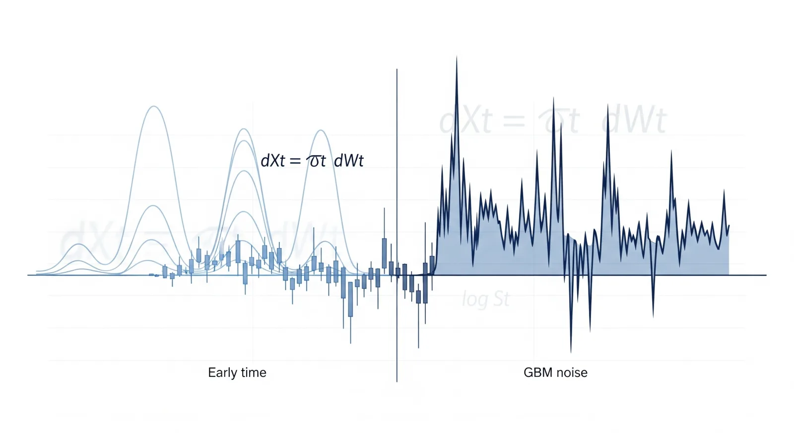
Kim, Choi, and Kim’s paper proposes a more finance-native diffusion design: use geometric Brownian motion (GBM) as an inductive bias in the forward noising process.1 The point is not to revive Black–Scholes as a complete market simulator. The point is narrower and more useful: make the noising process respect the fact that asset prices move multiplicatively and volatility scales with price level.
Operationally, the result is a synthetic-data generator that better reproduces three risk-relevant stylized facts: heavy-tailed returns, volatility clustering, and the leverage effect. In the paper’s tests, the empirical S&P 500 tail exponent is $\alpha = 4.35$; VE diffusion under linear and exponential schedules produces much lighter tails at $\alpha = 8.96$ and $\alpha = 8.49$, while GBM variants produce $\alpha = 3.06$, $4.62$, and $3.78$ across the tested schedules. Lower $\alpha$ means heavier tails, so this is not decorative statistics. It is the part of the distribution where risk teams normally discover their model has been wearing noise-cancelling headphones.
For business use, the immediate value is not “AI predicts the market”. Please, no. The value is more realistic synthetic trajectories for stress testing, VaR and Expected Shortfall experiments, scenario generation, and training-data augmentation. The boundary is equally important: the evidence is based on selected long-history S&P 500 daily data, not intraday order books, multi-asset portfolio dependence, live trading performance, or production-grade option pricing.
Markets are not pixels, regrettably
A standard diffusion model has an elegant ritual. Take clean data. Add noise step by step until the original structure is almost gone. Train a model to reverse the process. This has worked well in domains where the corruption process can be treated as broadly generic. Images tolerate a lot of Gaussian indignity.
Financial prices are less forgiving.
A stock price does not move like a greyscale pixel. A one-dollar move means something very different for a stock trading at $10 than for one trading at $1,000. The same absolute perturbation can be trivial in one regime and absurd in another. Financial time series also have persistent volatility, fat tails, and asymmetric volatility responses after negative returns. These features are not small aesthetic defects. They are the material from which risk systems, derivative books, and stress tests are built.
This is the paper’s useful starting point: the corruption process in a generative model is not neutral. If the forward noising process is structurally wrong for finance, the reverse process has to learn against a bad teacher. Larger networks may help, but only after the model has been asked the right question.
The authors’ answer is to move the financial structure into the noising mechanism itself.
The real move is noising log-prices, not simulating Black–Scholes
The most tempting misconception is that this paper simply wraps a neural network around Black–Scholes. That would be a neat way to generate a lot of synthetic data and an even neater way to generate disappointment.
The paper does something subtler. It uses GBM as an inductive bias for the forward diffusion process. In the Black–Scholes framework, an asset price follows a multiplicative stochastic process:
The key term is $\sigma_t S_t,dW_t$. Noise scales with the price. That is the financial intuition the authors want to preserve.
They then transform prices into log-prices, $X_t = \log S_t$. Applying Itô’s lemma gives:
By choosing $\mu_t = \frac{1}{2}\sigma_t^2$, the drift term disappears:
With $\sigma_t = \sqrt{\beta_t}$, the forward process becomes:
On the surface, this looks compatible with a variance-exploding score-based SDE in log-price space. In price space, however, the exponential mapping restores the finance-relevant behaviour: perturbations become state-dependent. High price levels receive proportionally larger absolute noise. The model does not need to pretend that every price level has the same uncertainty scale.
That is the mechanism-first contribution. The authors are not claiming GBM is the true law of markets. They are saying the noising process should at least respect the multiplicative skeleton of financial prices before the neural network starts its denoising performance.
A useful way to see the difference:
| Design choice | Generic diffusion habit | GBM-inspired diffusion choice | Why it matters |
|---|---|---|---|
| Where noise is applied | Generic numerical sequence | Log-price trajectory | Preserves multiplicative price structure |
| Noise behaviour | Additive | Price-proportional after mapping back to price space | Produces state-dependent volatility |
| Financial prior | Mostly absent | GBM-inspired | Builds finance structure into corruption, not only output checking |
| Main risk target | Sample realism in general | Heavy tails, volatility clustering, leverage | Aligns evaluation with risk-relevant market facts |
This is why the paper is more interesting than “diffusion, but for stocks.” It changes what the model is asked to destroy before it learns to reconstruct.
The score network still matters, but it is not the main character
The reverse process uses denoising score matching with a Transformer-based architecture adapted from Conditional Score-based Diffusion Imputation (CSDI). The architecture combines convolutional layers, temporal embeddings, Transformer blocks, gated residual modules, and skip connections. In plain English: local patterns, long-range temporal dependencies, and noise-level awareness all get representation capacity.
The authors also modify the architecture for financial series. The baseline CSDI-style setup uses 64 convolution channels, a 128-dimensional diffusion-step embedding, and a 16-dimensional feature embedding. That baseline can reproduce some heavy-tail and volatility-clustering behaviour, but it struggles with the leverage effect. The authors increase capacity to 128 convolution channels, 256-dimensional diffusion embeddings, and 64-dimensional feature embeddings.
This part of the paper is best read as an ablation and implementation refinement, not the core conceptual thesis. The main thesis is the GBM-inspired noising mechanism. The architecture experiment asks a narrower question: once the forward process is finance-aware, how much representational capacity is needed to capture asymmetric volatility responses?
The answer is: more than the vanilla CSDI settings. The 128/256/64 configuration gives the most stable leverage profiles across schedules, without the paper reporting obvious long-lag artifacts. That matters because leverage is harder than fat tails. Heavy tails ask whether extreme moves occur. Leverage asks whether bad returns and later volatility are temporally and asymmetrically linked. Markets enjoy being difficult like that.
The experimental setup tests the corruption mechanism, not just the generator
The experimental design compares three forward SDE families: VE, VP, and GBM. Each is tested under three noise schedules: linear, exponential, and cosine. For every configuration, the authors generate 120 synthetic time series, each of length $L = 2048$, and evaluate three stylized facts: heavy-tailed distributions, volatility clustering, and leverage effect.
The dataset comes from S&P 500 constituents. The authors remove problematic ticker symbols, download maximum available daily price histories through yfinance, and keep stocks with more than 40 years of available data. Daily log-returns are computed, then converted into overlapping subsequences with length 2048 and stride 400. The training setup uses minibatches of 64, trains for 1,000 epochs, sets the forward horizon to $T = 1$, and discretizes reverse diffusion into $N = 2000$ steps. The schedules use $\sigma_{\min}=0.01$ and $\sigma_{\max}=1.0$.
The design is not asking whether one trained model can win a leaderboard on one aggregate metric. It asks whether the forward noising process changes the kind of market structure the generator can reproduce.
That distinction matters because many synthetic-data systems fail in a boring way: the samples look plausible until you measure the statistics that traders and risk managers actually care about.
| Test | Likely purpose | What it supports | What it does not prove |
|---|---|---|---|
| Model-capacity variants | Ablation | Larger embeddings help capture leverage dynamics | That capacity alone explains the gains |
| VE/VP/GBM across schedules | Main evidence | Forward noising structure affects stylized-fact fidelity | Universal superiority across all markets |
| Heavy-tail exponent | Main evidence | GBM schedules better approximate empirical tail thickness | Accurate tail risk under all stress regimes |
| Volatility autocorrelation | Main evidence | GBM better preserves long-range volatility dependence | Correct volatility forecasting |
| Lead-lag leverage correlation | Main evidence | GBM better captures negative return / future volatility asymmetry | Tradable prediction signal |
| GAN comparison | Comparison with prior work | GBM diffusion is smoother and more stable on the tested stylized facts | Comprehensive benchmark against all modern financial generators |
This is a clean paper-reading rule: the figures are not interchangeable decorations. Figure 4 is a capacity ablation. Figures 5–7 are the main SDE-and-schedule evidence. Figure 8 is a comparison with prior GAN work. Mixing those categories would make the paper sound stronger and less precise. Tempting, but no.
Heavy tails: the model stops sanding off the dangerous part of the distribution
The first major result concerns return tails. In the real S&P 500 data used as the benchmark, the tail exponent is reported as $\alpha = 4.35$. In power-law language, a larger $\alpha$ means the tails decay faster. Faster decay means fewer extreme events. In finance, fewer extreme events is often what a model says right before reality invoices the balance sheet.
The VE SDE performs poorly under the linear and exponential schedules: $\alpha = 8.96$ and $\alpha = 8.49$. Those are far too light-tailed relative to the empirical benchmark. VE with a cosine schedule comes closer at $\alpha = 4.14$, but the paper’s broader evidence does not reduce to tail exponent alone.
The GBM SDE produces $\alpha = 3.06$, $4.62$, and $3.78$ across linear, exponential, and cosine schedules. The exponential and cosine schedules are closest to the empirical $\alpha = 4.35$, while the linear GBM schedule appears heavier-tailed than the benchmark.
The interpretation is straightforward. Additive noising tends to homogenize return magnitudes. It does not know that the uncertainty attached to a financial price should scale with the level of the price. GBM-inspired noising creates a channel for heteroskedasticity, so the generator has an easier path to producing extreme moves at realistic frequencies.
For operators, the lesson is not “choose GBM and stop checking tails.” It is: if synthetic market data underrepresents extremes, inspect the corruption process before worshipping the model architecture. The issue may not be model size. It may be that the model has been trained to clean the wrong kind of mess.
Volatility clustering: long memory needs more than pretty samples
Volatility clustering is the property that large moves tend to be followed by large moves and quiet periods tend to be followed by quiet periods. The sign may change; the magnitude persists. This is why a single turbulent day often changes risk limits for more than one day. The market does not politely reset at midnight.
The paper evaluates volatility clustering using autocorrelation of absolute log-returns. In empirical financial data, this autocorrelation tends to decay slowly with lag, often in a power-law-like pattern. VE diffusion, especially with a linear schedule, fails to retain this long-range dependence. The curve deteriorates sharply and can flatten or collapse unnaturally. VP is somewhat more stable in short-run dependence, but it shares the same broad additive-noise limitation.
GBM performs better, especially under exponential and cosine schedules. The paper reports a gradual and consistent decay in autocorrelation over several orders of magnitude in lag, closer to the empirical benchmark.
The schedule result is worth not over-reading. It does not mean exponential and cosine schedules have magical financial insight. It means the timing of noise injection interacts with the SDE choice. Linear noise growth can be too blunt. Exponential scheduling keeps early timesteps cleaner and increases noise more aggressively later. Cosine scheduling smooths the transition between low and high noise. When paired with a GBM structure, these schedules appear to preserve volatility dependence more effectively.
So the mechanism is two-layered. GBM supplies state-dependent perturbation. The schedule governs how quickly corruption escalates. The reverse model then learns to reconstruct trajectories from that structured degradation. Finance, as usual, refuses to let a single knob be enough.
Leverage is the hard test because it asks for asymmetry
Heavy tails and volatility clustering are necessary. They are not sufficient.
The leverage effect asks whether negative returns are followed by higher future volatility. This is an asymmetric temporal relationship. A generator can produce fat tails and clustered volatility and still fail to reproduce leverage. That failure matters for equity risk, volatility skew, and scenario generation. If synthetic data cannot encode the relationship between downside moves and later volatility, it will look calm in precisely the wrong places.
The paper measures leverage through lead-lag correlation between returns and future squared returns for lags $k = 0,\ldots,100$. VE shows only a mild leverage effect under the linear schedule, with a negative peak at $k=0$ that quickly fades and oscillates around zero. Under exponential and cosine schedules, VE becomes weaker and noisier. VP does not consistently capture the effect under any schedule.
GBM is stronger. All three GBM schedules show a strong negative correlation at $k=0$, with the cosine schedule dropping below $-5$ in the paper’s plotted scale. The authors note that this initial response may be amplified, but the correlation stabilizes and remains moderately negative across later lags.
This is also where the architecture ablation matters. The authors find that the vanilla CSDI-style model is not expressive enough to capture the asymmetric covariance structure between negative returns and later volatility. Increasing convolution channels and embedding dimensions improves the leverage profile. In other words, the forward process gives the model the right physics-flavoured hint; the score network still needs enough capacity to learn the asymmetry.
A cautious interpretation is better than a triumphant one. The result supports the claim that GBM-inspired diffusion can reproduce leverage-like structure more consistently than the tested baselines. It does not prove that the model has learned an economically stable causal mechanism. A negative lead-lag curve is a good diagnostic. It is not a trading oracle, despite what a pitch deck would do to it in the wrong hands.
The GAN comparison is useful, but not the final boss fight
The paper also compares the GBM-based diffusion model with a GAN-based financial time-series generator from prior work. The comparison again focuses on heavy tails, volatility clustering, and leverage.
The authors report that both the GAN and GBM diffusion reproduce heavy tails near the empirical benchmark, but GBM diffusion better captures the extreme tails. For volatility clustering, the GAN displays shorter-range dependence with noisier decay, while GBM diffusion shows a smoother and more persistent pattern. For leverage, the GAN produces erratic oscillations without a stable negative structure, while GBM diffusion produces a more consistent negative correlation.
This supports the paper’s main claim, but the comparison should not be stretched into a universal anti-GAN verdict. It is a comparison against a specific GAN approach and a specific evaluation setup. The more defensible takeaway is narrower: embedding financial structure into the diffusion noising process can outperform a prior neural generator on these stylized-fact diagnostics.
That is still useful. In financial data generation, fidelity is not just visual similarity. The generated series must preserve the statistical pathologies that make finance finance. Sadly, those pathologies are the product.
What the paper directly shows
The paper directly shows four things.
First, a GBM-inspired forward noising process can be expressed in log-price space in a way that aligns with variance-exploding score-based diffusion. That gives the method mathematical compatibility with existing score-based generative machinery.
Second, applying this idea to S&P 500 daily data improves reproduction of key stylized facts relative to VE and VP diffusion baselines. The improvement is clearest when GBM is paired with exponential or cosine schedules.
Third, model capacity matters for the leverage effect. The paper’s architecture ablation suggests that increasing convolutional and embedding dimensions improves the ability to learn asymmetric volatility responses.
Fourth, the GBM diffusion model compares favourably with the tested GAN baseline across the same stylized-fact diagnostics.
None of those statements requires claiming that the model prices options, forecasts returns, or understands macro regimes. Good. Those claims would need different evidence.
What Cognaptus infers for business use
The practical value is synthetic market data with better risk-relevant behaviour. That matters in at least four workflows.
| Business workflow | Practical use of better synthetic series | What this paper supports | Implementation boundary |
|---|---|---|---|
| Risk model testing | Generate return paths with heavier tails and clustered volatility | Stylized facts are better reproduced in daily S&P 500 experiments | Must still backtest VaR/ES exceedances on real holdout periods |
| Stress scenario design | Create plausible turbulent trajectories without relying only on historical replay | GBM diffusion preserves volatility persistence better than tested baselines | Does not guarantee coverage of unseen crisis mechanisms |
| Model augmentation | Expand training data for supervised financial models | Synthetic paths are statistically closer on selected diagnostics | Synthetic data can amplify model bias if used without validation |
| Derivatives diagnostics | Test sensitivity of pricing or hedging systems to path properties | Heavy tails, clustering, and leverage are relevant to options risk | No production option-pricing accuracy is demonstrated |
| Generator benchmarking | Evaluate whether a synthetic-data engine preserves market structure | The paper offers clear stylized-fact tests | Needs broader asset classes, frequencies, and dependency tests |
The most realistic near-term use is not replacing historical simulation. It is augmenting and probing it. Risk teams could use a model like this to generate controlled alternative histories, test whether downstream models break under clustered volatility, and compare synthetic stress paths against empirical crisis windows.
For AI-finance builders, the design principle is more important than the exact implementation: do not merely train a generic generator on financial data. Put market structure into the data corruption process, the conditioning variables, or the model architecture. Preferably all three, once the first one stops misbehaving.
The boundary: this is not a trading engine, pricing library, or exact GBM simulator
The paper is careful enough to state a limitation that many readers may miss. Although the model is GBM-inspired, it does not preserve exact log-normal marginal price distributions in the classical GBM sense. Classical GBM defines a Markovian continuous-time stochastic process with time-consistent log-normal marginals. This model jointly generates an entire learned log-price trajectory. The global sequence may reproduce stylized facts while individual marginals deviate from strict log-normality.
That is not a fatal flaw. It is a boundary. The model is a synthetic trajectory generator with a GBM-informed noising process, not a replacement for arbitrage-free derivative pricing machinery.
Other boundaries are equally important:
- The data are daily S&P 500 histories filtered for long availability. This is useful for broad equity-market regimes, but it does not establish performance on intraday data, illiquid assets, crypto, rates, FX, credit, or emerging-market equities.
- The model is evaluated on univariate-style stylized facts. Portfolio applications need cross-asset dependence, correlation breakdowns, sector co-movement, and tail dependence tests.
- The GAN comparison is informative but not exhaustive. Modern financial generative modelling includes many variants beyond the tested baseline.
- The paper does not demonstrate live forecasting, trading profitability, option-pricing accuracy, or hedging P&L improvement.
- The leverage effect result is encouraging but should be stress-tested across regimes and assets, especially because the strongest initial response appears amplified under cosine scheduling.
A synthetic-data model can be useful without being omniscient. In finance, that is not modesty. It is hygiene.
Better synthetic markets start with better corruption
The paper’s central contribution is not that GBM is perfect. It is that the forward noising process deserves financial discipline.
Most generative models focus attention on the reverse model: the Transformer, the score network, the denoiser, the architectural ornamentation. This paper reminds us that the first half of diffusion modelling is equally strategic. How you corrupt financial data determines what kind of reconstruction problem the model learns to solve.
If the corruption process treats prices as generic vectors, the model must recover market structure from a deliberately unfinancial degradation. If the corruption process respects multiplicative dynamics, the model starts from a better problem.
That is the business lesson. Synthetic finance does not get better merely by importing larger models from other domains. It gets better when the modelling assumptions stop pretending that markets are images with tickers attached.
Cognaptus: Automate the Present, Incubate the Future.
-
Gihun Kim, Sun-Yong Choi, and Yeoneung Kim, “A diffusion-based generative model for financial time series via geometric Brownian motion,” arXiv:2507.19003, 2025. https://arxiv.org/abs/2507.19003 ↩︎