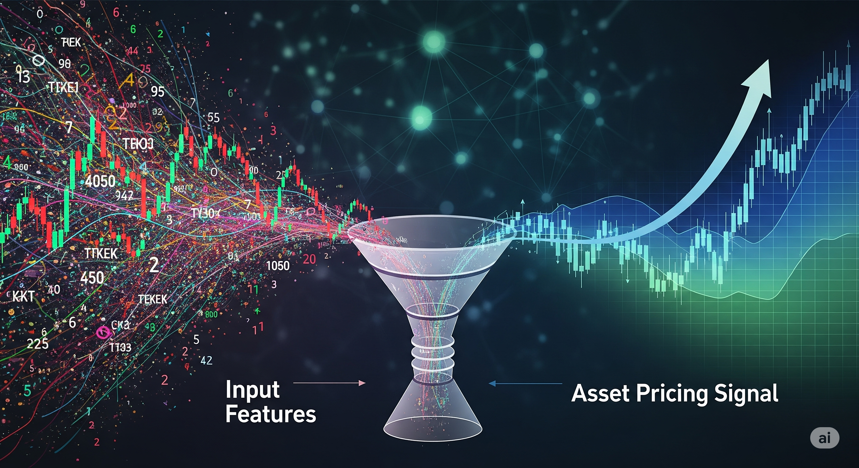
Deep learning has revolutionized many domains of finance, but when it comes to asset pricing, its power is often undercut by a familiar enemy: noise. Financial datasets are notoriously riddled with weak signals and irrelevant patterns, which easily mislead even the most sophisticated models. The result? Overfitting, poor generalization, and ultimately, bad bets.
A recent paper by Che Sun proposes an elegant fix by drawing inspiration from information theory. Titled An Information Bottleneck Asset Pricing Model, the paper integrates information bottleneck (IB) regularization into an autoencoder-based asset pricing framework. The goal is simple yet profound: compress away the noise, and preserve only what matters for predicting asset returns.
From Black Boxes to Bottlenecks
Traditional factor models like CAPM or Fama-French rely on hand-selected features, while machine learning models such as neural networks or random forests allow data to speak for itself. But with flexibility comes danger: as you increase the model’s capacity to capture non-linearities, you also increase its capacity to memorize irrelevant fluctuations.
That’s where the Information Bottleneck (Tishby et al., 2000) enters. It reframes learning as a trade-off:
- Minimize the mutual information I(Z; β) between the input features Z and the compressed latent representation β (to discard noise).
- Maximize the mutual information I(β; r) between the latent representation β and the asset returns r (to preserve signal).
This dual objective elegantly forces the model to forget unhelpful patterns while retaining the economically meaningful ones.
The optimization problem looks like this:
Variational methods are used to approximate the mutual information terms, making the model trainable via stochastic gradient descent.
When Bottlenecks Help (and When They Hurt)
The model is benchmarked against well-known approaches, including:
| Model | R^2@K=24 | Sharpe@K=24 |
|---|---|---|
| Fama-French | -11.4% | 0.60 |
| PCA | 1.6% | 0.33 |
| IPCA | 8.2% | 3.24 |
| CA1 (AutoEnc) | 7.6% | 3.42 |
| IPCA+IB | 9.9% | 3.63 |
| CA1+IB | 13.5% | 3.94 |
Key insights:
- For small factor models (K=1 to 3), the IB constraint can hurt performance. Why? Because when only a few factors are used, filtering aggressively may erase useful signal.
- For larger models (K=12 or 24), IB shines. It acts as a noise filter, allowing the deep network to explore rich non-linearities without overfitting.
This underscores an important lesson: regularization is not a universal good. Its benefits are architecture- and data-dependent.
Peeking Inside the Model
What makes this work more than just a table of results is the authors’ effort to visualize what the model learns. In particular:
- Mutual Information Tracking: As the depth of the beta network increases, mutual information with returns increases too—but only when IB is applied does this growth translate into better performance.
- Return Stability: During turbulent periods like the COVID-19 crash, models with IB regularization show more stable cumulative return curves and better Sharpe ratios, suggesting robust generalization rather than noise-chasing.

Implications for Practice
This approach isn’t just theoretical polish. It reflects a key pain point in asset management: the false promise of black-box ML. Sophisticated models often appear strong in-sample but crumble in deployment. The information bottleneck provides a principled way to penalize that complexity where it matters most.
If you’re building ML pipelines for financial prediction, especially with many input features (the paper uses 94), consider IB regularization as a core design element, not an afterthought. It doesn’t replace domain knowledge, but it does a fine job of enforcing a version of it: that not all data is created equal.
Cognaptus: Automate the Present, Incubate the Future