In a world where climate models span continents and economic simulators evolve across decades, it’s no longer enough to ask which variable affects the output the most. We must now ask: how does each input reshape the entire output distribution? The R package gsaot brings a mathematically rigorous answer, harnessing the power of Optimal Transport (OT) to provide a fresh take on sensitivity analysis.
The Sensitivity Analysis Bottleneck
Traditional global sensitivity analysis tools—like the popular Sobol’ indices—quantify how much variance in an output is driven by each input. But variance is a crude lens. What if two variables yield similar variances but one causes frequent outliers or fat tails? What if the outputs are multivariate, time-dependent, or spatially correlated? What if the inputs are correlated?
In such cases, variance-based tools stumble. They either simplify the problem (by reducing to a single output metric) or require costly sampling strategies with strong independence assumptions.
Optimal Transport to the Rescue
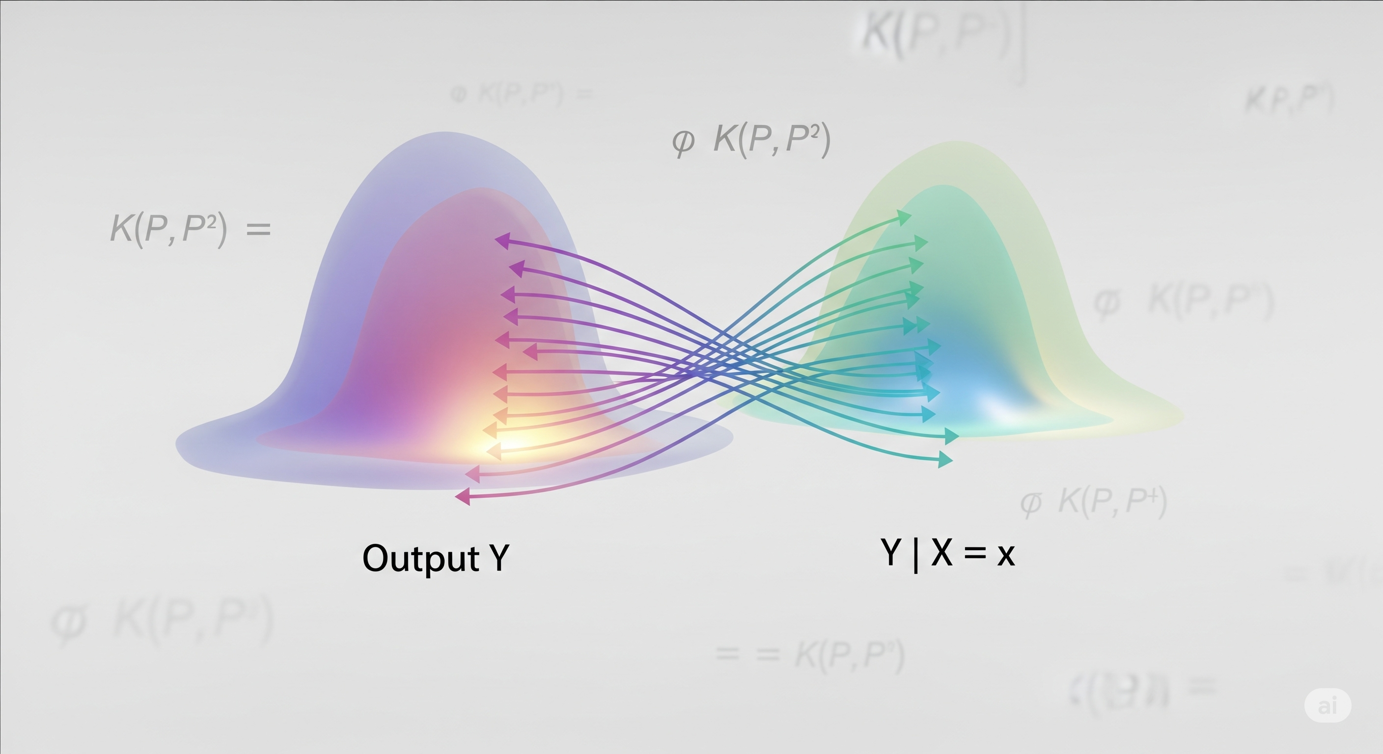
The Wasserstein distance, rooted in the theory of Optimal Transport, offers a more nuanced comparison between output distributions. Instead of comparing variances or means, it asks: what is the cost of morphing one distribution into another? This cost becomes a powerful sensitivity index: how much does fixing input $X_i$ deform the output distribution $Y$?
The authors of gsaot formalize this as:
$\iota_K(Y, X_i) = \frac{\mathbb{E}[W(P_Y, P_{Y|X_i})]}{\mathbb{E}[W(P_Y, P_{Y’})]}$
Where $W$ is the OT cost (e.g. squared Euclidean), and $P_Y$, $P_{Y|X_i}$ are marginal and conditional output distributions. This index satisfies:
- Zero-independence: zero if and only if $Y$ is independent of $X_i$.
- Max-functionality: one if $Y$ is a deterministic function of $X_i$.
- Normalization: always between 0 and 1.
Crucially, it works for multivariate outputs and correlated inputs.
Why gsaot Matters
The gsaot package takes these theoretical advances and makes them accessible:
- Model-agnostic: It works on any input-output dataset, including black-box models.
- Multivariate and correlated-ready: No simplification needed.
- Solver-flexible: Choose between exact OT (network simplex, Bures) or fast approximations (Sinkhorn).
- Decomposable insights: Break down effects into mean (advective), variance (diffusive), and higher-order contributions.
- Visual diagnostics: Local separation plots highlight input impact across their domain.
Comparison: OT Indices vs Traditional Methods
| Feature | Sobol' | gsaot OT Indices |
|---|---|---|
| Handles multivariate outputs | No | Yes |
| Requires input independence | Yes | No |
| Interpretable in probability | Limited | Strong (via distributions) |
| Supports arbitrary models | Often No | Yes (post-hoc dataset use) |
| Bootstrap CIs & ranking | Varies | Built-in |
Use Cases That Shine
🌲 Spruce Budworm & Forest Model
Time-dependent ODEs with 3 outputs (budworm population, tree size, energy reserve). OT indices captured the influence of growth parameters across time, revealing that central values of inputs like $K$ and $r_s$ have minimal effect—a nuance missed by Sobol-type variance indices.
🌍 DICE Climate Model
Tracking atmospheric temperature anomaly from 2015 to 2100, the authors applied custom cost functions using Minkowski distance ($L^3$), showing how parameters like climate sensitivity $S$ and forcing $\lambda$ shift temperature trajectories. Dummy variables confirmed others could safely be fixed.
📈 Gaussian Linear Test Case
With known ground truth, the package accurately recovered Wasserstein-Bures index values and decomposed them into mean and covariance contributions.
Practical Considerations
- Speed: Fast closed-form estimators exist for 1D and elliptical Gaussian outputs.
- Sample Size: Robust for $N \geq 1000$, with minimal tuning of partition count $M$.
- Numerical Noise Check: Use a dummy variable to benchmark irrelevance.
- Parallel Bootstrap: Built-in, customizable with
futureandbootintegration.
The Bigger Picture
As model complexity grows, so must our tools for understanding them. The gsaot package shows how Optimal Transport isn’t just a mathematical curiosity; it’s a practical upgrade to the statistical machinery behind risk assessment, policy evaluation, and simulation analysis.
Instead of asking how much an input affects the output, it invites us to ask: how does an input reshape reality? That’s a better question. And gsaot helps us answer it.
Cognaptus: Automate the Present, Incubate the Future