In the paper Deep Reinforcement Learning for Urban Air Quality Management: Multi-Objective Optimization of Pollution Mitigation Booth Placement in Metropolitan Environments, Kirtan Rajesh and Suvidha Rupesh Kumar tackle an intricate urban challenge using AI: where to place air pollution mitigation booths across a city to optimize overall air quality under multiple, conflicting objectives1.
The proposed solution uses Proximal Policy Optimization (PPO), a modern deep reinforcement learning algorithm, and a multi-dimensional reward function to model this real-world spatial optimization. But beneath the urban context lies a mathematical and algorithmic structure that holds powerful potential for business decision-making—especially where trade-offs between objectives are crucial.
The AI Under the Hood: PPO and Multi-Dimensional Reward Functions
PPO: Stabilized Policy Gradient
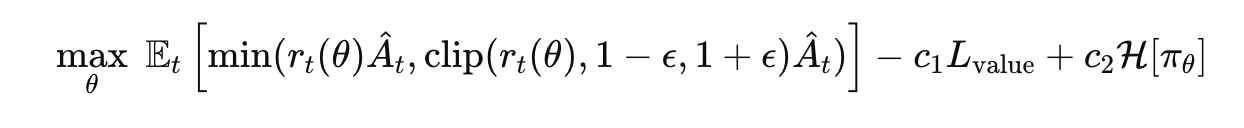
The PPO method used in the paper is grounded in the trust-region approach. The central loss function combines the clipped objective with value and entropy terms:
$$ L(\theta) = \mathop{\mathbb{E}}\limits_{t}\bigl[ L_{\mathrm{CLIP}}(\theta) - c_1 L_{\mathrm{value}} + c_2 L_{\mathrm{entropy}} \bigr] $$
Where:
- $L_{\text{CLIP}}(\theta) = \mathbb{E}_t \left[ \min\left( r_t(\theta) \hat{A}_t, \text{clip}(r_t(\theta), 1 - \epsilon, 1 + \epsilon) \hat{A}_t \right) \right]$
- $r_t(\theta) = \frac{\pi_\theta(a_t | s_t)}{\pi_{\theta_{\text{old}}}(a_t | s_t)}$
- $L_{\text{value}} = \frac{1}{N} \sum_t (V_\theta(s_t) - R_t)^2$
- $L_{\text{entropy}} = -\sum_a \pi_\theta(a|s) \log \pi_\theta(a|s)$
In the original paper, the policy network $\pi_\theta$ is implemented as a CNN that takes spatial inputs (like pollution heatmaps) and transforms them into action probabilities for booth placement. Thus, $\theta$ includes all CNN weights.
Training occurs end-to-end: PPO gradients flow from the reward loss back through the CNN layers to adapt feature maps to real-world outcomes.
Generalized PPO for Business Decision-Making
This version abstracts the architecture (CNN, MLP, Transformer) and makes $s_t$ a general representation of the business environment (customer profile, market state, etc.).
Multi-Dimensional Rewards (with Constraints)
In the original paper:
$$ R(s_t, a_t) = w_1 R_{\text{local}} + w_2 R_{\text{global}} + w_3 R_{\text{pop}} + w_4 R_{\text{traffic}} + w_5 R_{\text{ind}} $$
Constraint violations are not treated as additive penalties but enforced via feasibility masks:
$$ \mathbb{I}_{\text{valid}}(a_t) = \begin{cases} 1 & \text{if action is feasible} \ 0 & \text{if constraint is violated} \end{cases} $$
Final reward becomes:
$$ R^*(s_t, a_t) = R(s_t, a_t) \cdot \mathbb{I}_{\text{valid}}(a_t) $$
Generalized Reward Function for Business
For richer modeling:
$$ R(s_t, a_t) = \Phi\left(\sum_{i=1}^n w_i R_i(s_t, a_t)\right) \cdot \mathbb{I}_{\text{valid}}(a_t) $$
Where:
- $R_i$: Component reward (e.g., sales, brand sentiment, operational efficiency)
- $w_i$: Dynamic or state-conditioned weight
- $\Phi(\cdot)$: Nonlinear transformation (log, softplus, sigmoid)
- $\mathbb{I}_{\text{valid}}$: Constraint gate (e.g., budget, regulation)
Model Variants for Business Use
1. Generalized Advantage Estimation (GAE)
Purpose: Smooth advantage estimation to reduce variance without increasing bias significantly.
Mechanism: Instead of calculating return-to-go directly, GAE computes advantage with exponential decay:

Where $\delta_t = r_t + \gamma V(s_{t+1}) - V(s_t)$. Parameters $\gamma \in [0, 1]$, $\lambda \in [0, 1]$.
Pros:
- Provides smoother gradients
- Improves training stability
Cons:
- Sensitive to $\lambda$ and $\gamma$ tuning
2. Multi-Agent PPO
Purpose: Coordinate decisions from different actors (e.g., departments, retail locations).
Mechanism: Each agent $i$ has its own policy $\pi_\theta^i$, and receives its own reward $R^i$, possibly augmented by shared global objectives:
$$ R^i = R^i_{\text{local}} + \eta R_{\text{global}} $$
Pros:
- Models distributed decision-makers
- Encourages competition/cooperation among agents
Cons:
- Credit assignment becomes difficult
- Computational complexity increases significantly
3. Hierarchical PPO
Purpose: Separate strategic decisions (long-term) and tactical actions (short-term).
Mechanism: High-level policy selects sub-goals; low-level policy selects atomic actions to fulfill them:
$$ \pi_{\text{high}}(g|s), \quad \pi_{\text{low}}(a|s, g) $$
Pros:
- Modular design fits multi-scale business needs
- Enhances interpretability
Cons:
- Requires reward design at both levels
- Harder to train and debug
Full PPO + Multi-Reward Training Code (Python and R)
Python Implementation
# Define environment and policy
env = BusinessEnv()
policy = PolicyNetwork()
value_fn = ValueNetwork()
optimizer = torch.optim.Adam(policy.parameters(), lr=3e-4)

# PPO hyperparameters
EPISODES = 500
update_epochs = 10
c1, c2, eps = 0.5, 0.01, 0.2

# GAE
 def compute_GAE(traj, value_fn, gamma=0.99, lam=0.95):
    values = value_fn(traj.states)
    deltas = traj.rewards + gamma * torch.roll(values, -1) - values
    advantages = []
    adv = 0.0
    for delta in reversed(deltas):
        adv = delta + gamma * lam * adv
        advantages.insert(0, adv)
    return torch.tensor(advantages)

# Collect trajectories
 def collect_trajectory(policy, env):
    states, actions, rewards, old_probs = [], [], [], []
    state = env.reset()
    done = False
    while not done:
        prob = policy(state)
        action = sample_from(prob)
        next_state, reward, done = env.step(action)

        states.append(state)
        actions.append(action)
        rewards.append(reward)
        old_probs.append(prob[action])

        state = next_state
    return Trajectory(states, actions, rewards, old_probs)

# Training loop
for episode in range(EPISODES):
    traj = collect_trajectory(policy, env)
    advantages = compute_GAE(traj, value_fn)

    for _ in range(update_epochs):
        ratio = (policy(traj.states, traj.actions) / traj.old_probs)
        clip_obj = torch.min(ratio * advantages, torch.clamp(ratio, 1-eps, 1+eps) * advantages)
        value_loss = (value_fn(traj.states) - compute_returns(traj.rewards)).pow(2).mean()
        entropy = -(policy * torch.log(policy)).sum(dim=-1).mean()

        total_loss = -clip_obj.mean() + c1 * value_loss - c2 * entropy
        optimizer.zero_grad()
        total_loss.backward()
        optimizer.step()
R Implementation
ppo_train <- function(policy, value_fn, env, episodes = 500) {
  for (ep in 1:episodes) {
    traj <- collect_trajectory(policy, env)
    adv <- compute_gae(traj, value_fn)

    for (epoch in 1:10) {
      ratio <- policy$prob(traj$states, traj$actions) / traj$old_probs
      clipped <- pmin(ratio * adv, pmax(1 - 0.2, pmin(ratio, 1 + 0.2)) * adv)
      value_loss <- mean((value_fn$predict(traj$states) - traj$returns)^2)
      entropy <- -mean(policy$entropy(traj$states))

      total_loss <- -mean(clipped) + 0.5 * value_loss - 0.01 * entropy
      policy$update(total_loss)
    }
  }
}

collect_trajectory <- function(policy, env) {
  states <- actions <- rewards <- old_probs <- list()
  state <- env$reset()
  done <- FALSE
  while (!done) {
    prob <- policy$predict(state)
    action <- sample(seq_along(prob), 1, prob = prob)
    res <- env$step(action)
    next_state <- res$state
    reward <- res$reward
    done <- res$done

    states <- append(states, list(state))
    actions <- append(actions, action)
    rewards <- append(rewards, reward)
    old_probs <- append(old_probs, prob[action])

    state <- next_state
  }
  list(states = states, actions = actions, rewards = rewards, old_probs = old_probs)
}

compute_gae <- function(traj, value_fn, gamma = 0.99, lambda = 0.95) {
  values <- value_fn$predict(traj$states)
  deltas <- mapply(function(r, v, vp) r + gamma * vp - v,
                   traj$rewards, values, c(values[-1], 0))
  adv <- numeric(length(deltas))
  adv[length(deltas)] <- deltas[length(deltas)]
  for (t in (length(deltas) - 1):1) {
    adv[t] <- deltas[t] + gamma * lambda * adv[t + 1]
  }
  adv
}
PPO in Business Setup #1: Retail Pricing Strategy
- State ($s$): previous sales volume, stock level, seasonality
- Action ($a$): price for SKU
- Reward ($R$): based on margin, volume, and complaints
- Policy: neural network outputs price probability distribution
Steps:
- Simulate customer response to different prices
- Compute reward via multi-dimensional function
- Estimate $\hat{A}_t$ via GAE
- Apply PPO update with clipped objective
PPO in Business Setup #2: Logistics Routing
- State ($s$): includes current vehicle location, time of day, weather conditions, and package urgency level
- Action ($a$): select the next route segment or delivery sequence to follow
- Policy: neural network policy $\pi_\theta(a|s)$ maps state to route decision probabilities
Mathematical Reward Expression
We define the reward as a composite of delivery performance:
$$ R(s_t, a_t) = -\alpha_1 \times \text{Time}(a_t) - \alpha_2 \times \text{FuelCost}(a_t) + \alpha_3 \times \text{Reliability}(a_t) - \lambda_1 \times I_{\text{late}}(a_t) $$
Where:
- Time($a_t$): estimated delivery time in hours
- FuelCost($a_t$): cost in dollars
- Reliability($a_t$): historical success rate for that path
- $I_{\text{late}}(a_t)$: binary indicator (1 if delivery is late, 0 otherwise)
- Example parameters: $\alpha_1 = 0.5$, $\alpha_2 = 0.3$, $\alpha_3 = 0.2$, $\lambda_1 = 50$
Example Calculation
Suppose:
- Time = 6 hours
- FuelCost = 120 dollars
- Reliability = 0.95
- $I_{\text{late}} = 0$ (on time)
Then:
$$ R = -0.5 \times 6 - 0.3 \times 120 + 0.2 \times 0.95 = -3 - 36 + 0.19 = -38.81 $$
PPO in Business Setup #3: Campaign Allocation
- State: market segment, time of day, platform saturation, remaining budget
- Action: choose advertising channel (e.g., TikTok, Facebook, Email)
- Policy: neural network $\pi_\theta(a|s)$ outputs distribution over ad channels
Mathematical Reward Expression
We define the reward based on conversion efficiency, cost, and sentiment uplift:
$$ R(s_t, a_t) = \alpha_1 \times \text{ConvRate}(a_t) - \alpha_2 \times \text{CPA}(a_t) + \alpha_3 \times \text{SentimentLift}(a_t) - \lambda_1 \times I_{\text{overbudget}}(a_t) $$
Where:
- ConvRate($a_t$): observed conversion rate after placing ads on channel $a_t$
- CPA($a_t$): cost per acquisition (dollars)
- SentimentLift($a_t$): increase in brand sentiment from channel $a_t$
- $I_{\text{overbudget}}(a_t)$: indicator for exceeding budget (1 if exceeded, else 0)
- Typical values: $\alpha_1 = 0.5$, $\alpha_2 = 0.4$, $\alpha_3 = 0.1$, $\lambda_1 = 100$
Example Calculation
Suppose:
- ConvRate = 0.04 (4%)
- CPA = 25 USD
- SentimentLift = 3.2 (on a scale of -5 to +5)
- No budget overrun ($I_{\text{overbudget}} = 0$)
Then:
$$ R = 0.5 \times 0.04 - 0.4 \times 25 + 0.1 \times 3.2 = 0.02 - 10 + 0.32 = -9.66 $$
Final Thoughts
By borrowing mathematical structures from urban optimization—especially PPO with constraint-aware, multi-dimensional rewards—businesses can model decisions in richly nuanced ways. This approach balances multiple goals, adapts through learning, and ultimately leads to better, data-driven strategy formation.
-
arXiv:2505.00668 Deep Reinforcement Learning for Urban Air Quality Management: Multi-Objective Optimization of Pollution Mitigation Booth Placement in Metropolitan Environments Kirtan Rajesh, Suvidha Rupesh Kumar ↩︎