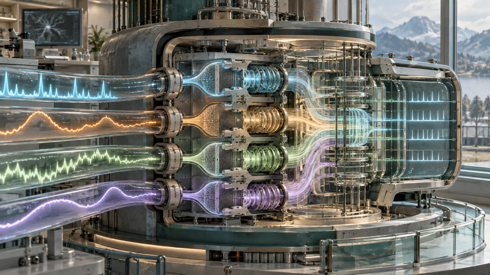
TL;DR for operators
Scientific instruments can measure the same underlying activity while producing signals with different response times, noise patterns, and temporal distortions. Maintaining a separate predictive model for every sensor is one solution, but it becomes increasingly difficult to manage as measurement technologies diversify.
SpikeSSL1 offers an alternative: one neural architecture that adjusts its temporal processing according to the characteristics of each recording. Across five held-out evaluation conditions, it achieves mean spike-rate correlation of 0.654 versus 0.483 for the strongest competing baseline. Biophysical simulation improves its five-seed average to 0.708, although individual conditions do not benefit equally.
For neuroscience analytics and scientific instrument software, the implication is a potentially more reusable inference engine. The qualification is substantial: sensor adaptation does not eliminate recording artifacts, calibration requirements, or the need for condition-specific validation.
Different sensors change what the same signal means
Consider an analytics platform receiving calcium-imaging recordings from several laboratories. Each laboratory measures neuronal activity, but the sensors can respond differently to the same underlying sequence of electrical spikes.
Some calcium indicators produce relatively rapid fluorescence responses. Others decay more slowly, allowing signals from successive spikes to overlap. Measurement noise, saturation, sampling frequency, and biological preparation introduce further differences.
The inference problem is therefore more complicated than recognizing a recurring pattern in a time series. The model must reconstruct neuronal activity from measurements whose temporal behavior depends partly on the sensor producing them.
A model trained on one indicator may mistake the lingering fluorescence from an earlier spike for evidence of continuing activity. Conversely, it may miss closely spaced spikes when their responses merge.
A conventional approach is to train or calibrate separate models for different acquisition conditions. Another is to combine more training data and increase model capacity.
SpikeSSL investigates a third possibility: can a shared model learn common neuronal-response structure while adapting its temporal interpretation to each input?
This question matters because adding observations from unfamiliar sensors does not necessarily teach a generic network how the measurement process works.
A shared model whose memory changes with the recording
The architecture begins with a physical property of calcium fluorescence: its response to a spike often persists and gradually decays.
SpikeSSL represents this persistence using infinite-impulse-response (IIR) state-space layers. Each layer maintains an internal state that combines historical information with new measurements:
Here, $h_t$ is the current hidden state, $z_t$ is the incoming representation, and $\alpha$ controls how much historical information is retained.
Different channels learn different decay coefficients, allowing the network to represent several temporal scales. Forward and backward processing capture both preceding activity and the subsequent fluorescence response.
This is an inductive bias motivated by calcium dynamics, not a complete mathematical reconstruction of every biochemical process governing fluorescence.
The more distinctive feature is that these temporal coefficients need not remain fixed across inputs.
SpikeSSL combines indicator identity, sampling frequency, and seven signal statistics—including variability, distributional shape, and autocorrelations—into a conditioning representation. This representation adjusts both the recurrent decay coefficients and feature normalization through Adaptive Layer Normalization (AdaLN).
A slow-decaying, highly autocorrelated recording can consequently receive different temporal processing from a faster recording, even though both pass through the same trained architecture.
In zero-shot testing, the held-out indicator is assigned an unknown identity rather than supplied with its true sensor label. The model still uses the current recording’s sampling information and independently computed window statistics. It does not require target labels, pooled target recordings, or parameter updates.
That distinction is central. A shared model does not have to apply identical processing to every sensor. It can share learned structure while modifying how that structure operates.
The benchmark favors appropriate dynamics over parameter count
The authors evaluate SpikeSSL on public paired fluorescence and electrophysiological recordings, reporting 33 datasets and 1,960 neuron recordings across 11 calcium indicators.
They use five fixed evaluation conditions. In-domain tests include recordings from the relevant conditions during training, while reserving evaluation recordings. Zero-shot leave-one-indicator-out (LOIO) tests remove the designated source-side indicator or recording family from training.
The principal metric is Pearson correlation between inferred and ground-truth spike rates. Higher correlation indicates better reconstruction of temporal variation, although it does not independently establish accurate spike counts or eliminate mean-rate bias.
| Evaluation or intervention | Mean correlation |
|---|---|
| SpikeSSL, in-domain | 0.741 |
| ENS2, in-domain | 0.545 |
| SpikeSSL, zero-shot LOIO | 0.654 |
| ENS2, zero-shot LOIO | 0.483 |
| SpikeSSL without bidirectional IIR, zero-shot | 0.594 |
| SpikeSSL without AdaLN, zero-shot | 0.601 |
Sources: main Tables 1–2 and component-ablation Table 4. The ablations are single-seed comparisons.
The zero-shot advantage over ENS2 is 0.171 correlation points. More revealing are the component-removal experiments: replacing the dynamics-informed IIR backbone reduces mean correlation by 0.060, while removing adaptive normalization reduces it by 0.053.
These are ablation tests, not independent deployment trials. Their purpose is to establish whether the proposed components contribute within a controlled benchmark. Both interventions weaken performance.
Parameter-budget comparisons reinforce the architectural interpretation. A larger ENS2 variant with 4.2 million parameters reaches 0.564 correlation, while SpikeSSL reaches 0.654 with approximately 3.9 million parameters.
Simply enlarging the conventional baseline does not reproduce the result.
The finding does not establish that physical inductive biases always outperform scaling. It shows that, for these calcium-inference conditions, the structure of temporal processing contributes information that additional parameters alone do not recover.
The evaluation groups also require careful interpretation. They include related GCaMP8 variants and a brain-to-spinal-cord transfer condition, rather than five entirely novel molecular sensor families.
Synthetic fluorescence expands coverage, but not uniformly
Real recordings with simultaneous fluorescence and electrical ground truth are expensive to obtain and unevenly distributed across indicators.
SpikeSSL addresses this limitation with approximately 11,000 synthetic training traces. The simulator generates spike activity and transforms it into fluorescence using calcium decay, response depletion and recovery, nonlinear indicator binding, baseline drift, and measurement noise.
These synthetic recordings augment training; they are not included in the evaluation recordings.
In the main single-seed comparison, simulation raises mean zero-shot correlation from 0.654 to 0.704. Across five random seeds, the corresponding averages improve from 0.660 ± 0.016 to 0.708 ± 0.011.
The condition-level results reveal why the average needs qualification.
| Held-out condition | Five-seed change in mean correlation |
|---|---|
| V1-OGB | +0.038 |
| V1-GCaMP6s | +0.024 |
| V1-GCaMP8 | +0.050 |
| Other-RCaMP | −0.012 |
| SC-GCaMP6s | +0.138 |
Source: Appendix A.14, Table 20.
The spinal-cord condition benefits substantially. Other-RCaMP does not improve on average, although its small negative change lies within reported variability and does not establish conclusive harmful transfer.
The appendix also examines whether simulation makes training and target signal distributions more similar. Improved alignment does not consistently translate into higher reconstruction accuracy.
This gives simulation a narrower but more credible role: it can expand coverage of plausible sensor behavior, but its value depends on whether simulated dynamics resemble those that matter for the target recordings.
There is also a reporting boundary. A supplementary progressive loss-ablation table reports 0.660 for its full simulation-augmented configuration, rather than the main comparison’s 0.704. The supplied research record does not reconcile these values or establish identical experimental setups, so they should not be treated as interchangeable.
What a shared inference engine would change
For a neuroscience analytics platform, the immediate design question is whether a pooled, condition-aware inference engine can become the default processing method across supported sensors.
SpikeSSL suggests three practical requirements.
First, the platform must retain acquisition metadata and extract meaningful signal statistics. These inputs directly influence model behavior; they are not merely descriptive information attached after inference.
Second, model validation should preserve sensor-specific and preparation-specific results. A strong pooled average can conceal weaker transfer to particular indicators or tissues. Synthetic training should be evaluated against each intended acquisition regime rather than approved solely on overall improvement.
Third, the system should distinguish estimated neuronal activity from confidence in that estimate. SpikeSSL includes a binary activity gate and a heteroscedastic variance head that estimates frame-level uncertainty. Within the benchmark, higher predicted variance is associated with larger errors and held-out conditions.
That association provides a potential quality-monitoring signal, but it does not establish universally calibrated uncertainty or a clean separation between measurement noise and uncertainty about the model itself.
These are architectural and validation implications drawn by Cognaptus from the research. The paper does not measure reductions in software maintenance expenditure, calibration costs, or laboratory operating time.
Acquisition artifacts remain a separate reliability problem
The clearest deployment boundary appears in the acquisition-robustness experiments.
Under the tested baseline-drift perturbation, mean zero-shot correlation drops from 0.654 to 0.555. Sparse motion artifacts also reduce performance, although less severely in the reported comparison.
Input-conditioned temporal processing therefore does not make the model insensitive to non-biological changes in the signal. Motion correction, baseline detrending, and recording-quality checks remain relevant upstream controls.
The bidirectional architecture introduces another constraint: inference uses future fluorescence observations within a processing window. That makes it suitable primarily for offline analysis or workflows able to tolerate future-context requirements, rather than strictly causal real-time inference.
Finally, the experiments establish predictive comparisons on a heterogeneous but finite benchmark. They do not show that one trained model can reliably handle every future indicator, acquisition technology, or experimental preparation.
For teams evaluating adoption, the appropriate sequence is to validate known sensor conditions, test explicitly held-out acquisition regimes, examine artifact sensitivity, and only then determine where calibration or targeted adaptation remains necessary.
Universal architecture, conditional reliability
SpikeSSL’s contribution is a concrete demonstration that shared predictive models can benefit from adapting their internal dynamics to the measurement process.
The IIR backbone supplies multiple temporal memory scales. Conditioning changes how those scales operate for each recording. Biophysical simulation broadens the training distribution where paired observations are scarce.
Together, these choices outperform conventional comparators across the paper’s selected benchmark conditions. Yet their effectiveness remains dependent on the sensor dynamics, training coverage, and quality of the incoming recordings.
For scientific software developers, the consequential shift is from maintaining a separate inference model for every sensor toward maintaining a shared architecture with explicit acquisition-aware behavior and condition-specific validation.
The result is a promising strategy for making inference systems more reusable—not evidence that the underlying measurement differences have disappeared.
Cognaptus: Automate the Present, Incubate the Future.
-
Chenghao Yue and Siming Xing and Shuran Liu and Angran Li and Yuanlong Zhang (2026). SpikeSSL: A Universal Spike Inference Framework with Dynamics-Informed State-Space Layers. arXiv:2610.11456. https://arxiv.org/abs/2610.11456 ↩︎