TL;DR for operators
A recent paper on warehouse planning uses knowledge graphs and LLM reasoning to diagnose bottlenecks in discrete-event simulation outputs.1 The useful part is not that someone put a chatbot on top of a warehouse model. That would be adorable, and mostly useless. The useful part is that the authors first make simulation traces structurally queryable, then force the LLM to investigate in steps.
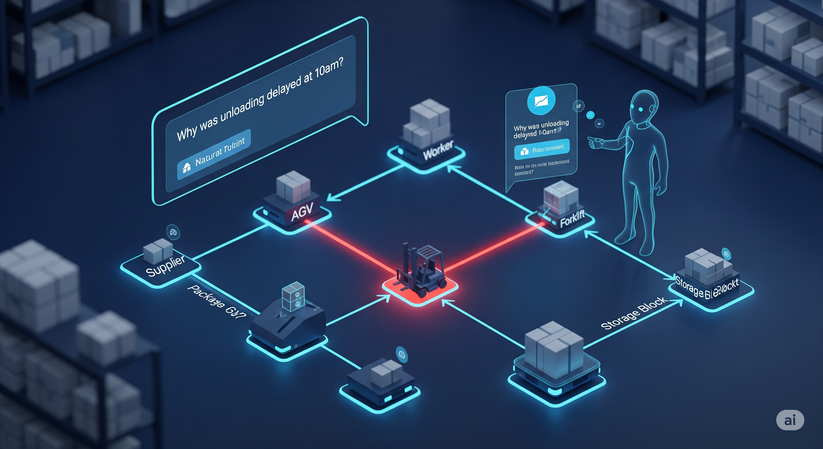
The system converts DES event logs into a knowledge graph containing suppliers, workers, AGVs, forklifts, storage blocks, and package movement relationships. The LLM then generates Cypher queries, checks intermediate answers, and builds a diagnosis from evidence rather than producing one grand, fragile answer from a single prompt.
On 25 operational questions, the paper reports average Pass@1/Pass@4 scores of 0.82/1.00 for the Step-wise Guide method, compared with 0.41/0.56 for direct QA and 0.73/0.80 for direct QA with self-reflection. In plain operator language: decomposing the question before querying the graph makes the system much less likely to grab the wrong timestamp, path, or aggregation.
The bottleneck case studies are more important than the headline number. The agent identifies an AGV-to-forklift transfer delay for CamelCargo, supplier-linked slowdown around AuroraFarms, and degraded forklift performance around FL_00. These are not magic discoveries. They are structured investigations over timestamped process evidence. That is precisely why they are useful.
The business implication is narrower, and better, than the usual AI pitch. This is a way to make simulation output easier to interrogate, audit, and turn into interventions. It is not yet a general warehouse brain. The evidence is from an in-house unloading simulation, with a custom graph schema and qualitative bottleneck evaluation. Good tool. Not a forklift oracle. Let us all try to remain adults.
Bottlenecks are not always hidden; sometimes they are just badly indexed
Every warehouse operator knows the meeting.
Something ran slow. Someone has a dashboard. Someone else has a spreadsheet. The simulation analyst has event logs. The floor manager remembers that one forklift looked suspicious. The planning team asks the innocent question: “What caused the delay?”
Then the room discovers that “delay” is not a metric. It is a crime scene.
A supplier may have waited before unloading. Workers may have been underused. AGVs may have arrived late. Forklifts may have been occupied, slow, badly sequenced, or simply accused because they were nearest to the evidence. Packages may have followed different paths through the facility. Aggregate averages can point toward the smoke, but they rarely tell you which wire burned first.
This is the problem the paper attacks. Discrete-event simulation is already good at generating detailed operational traces. It can record when suppliers arrive, when workers pick packages, when AGVs begin and end journeys, when forklifts receive packages, and when storage placement finishes. The awkward part is interpretation. A simulation can produce a huge amount of truth in a format that humans do not enjoy reading. Classic enterprise software behaviour, really.
The paper’s answer is mechanism-first: before asking an LLM to explain a bottleneck, restructure the simulation output into a knowledge graph. Then make the LLM reason through that graph using targeted Cypher queries, intermediate checks, and step-by-step decomposition.
That order matters. Without the graph, the LLM is mostly a fluent narrator. With the graph, it becomes a query planner, evidence collector, and summariser over a structured operational trace. Still fallible, obviously. But now at least it has something firmer than vibes.
The mechanism: make the simulation queryable before making it conversational
The simulated warehouse process in the paper is an unloading and storage flow. Supplier trucks arrive with packages. Workers move packages from suppliers to waiting points. AGVs carry packages onward to forklift pickup points. Forklifts place packages into storage. The DES captures process and equipment-specific timestamps, plus package-level timestamps across the handling path.
The authors turn this output into a graph. The graph schema is deliberately operational rather than decorative. Nodes represent entities such as:
| Node type | Operational role |
|---|---|
SUPPLIER |
Truck or supplier source, with arrival and discharge timestamps |
WORKER |
Human unloading resource |
AGV |
Automated guided vehicle moving packages through the facility |
FL |
Forklift handling final placement |
STORAGE |
Destination storage block |
The relationships carry the package flow and timestamps:
| Relationship | What it represents |
|---|---|
SUPPLIER_TO_WORKER |
Package handoff from supplier-side unloading to worker handling |
WORKER_TO_AGV |
Worker handoff to AGV, including AGV arrival and journey start timestamps |
AGV_TO_FL |
AGV arrival at forklift stage and forklift placement start |
FL_TO_STORAGE |
Forklift placement completion into storage |
This is the first important design choice. The system is not merely dumping logs into a vector database and asking the model to “find relevant chunks.” It is mapping the simulated operational process into a graph where paths, timestamps, and resource relationships can be queried directly.
A simplified view looks like this:
DES event logs
   ↓
Knowledge graph of resources, packages, timestamps, and process relationships
   ↓
Natural-language question
   ↓
Query classification
   ↓
Operational QA chain OR investigative reasoning chain
   ↓
Step-wise Cypher queries + execution + correction + self-reflection
   ↓
Evidence-linked answer or bottleneck diagnosis
That pipeline is the paper’s real contribution. Not the presence of GPT-4o. Not the fact that Cypher appears. Not the word “agent,” which now gets attached to anything that survives three API calls without supervision. The contribution is the control structure: decompose, query, check, continue.
For routine operational questions, the system uses a QA chain. It breaks the user’s question into structured steps, generates Cypher for each step, executes those queries against Neo4j, corrects errors, and synthesises an answer.
For investigative bottleneck questions, it uses an iterative reasoning chain. The agent asks one sub-question at a time, uses the answer to choose the next investigative step, and stops when it has gathered enough evidence to produce a diagnosis.
That distinction is valuable. “Which supplier had the shortest discharge time?” is not the same kind of task as “Why was discharge slow between 10:00 and 12:30?” The first is retrieval plus aggregation. The second is forensic analysis.
Trying to solve both with one giant query is how software becomes expensive theatre.
Why step-wise querying beats heroic single-shot Cypher
The operational QA experiment tests 25 questions across suppliers, workers, AGVs, forklifts, and packages. The authors compare three methods:
| Method | How it works | Average Pass@1 | Average Pass@4 |
|---|---|---|---|
| Direct QA | Single-pass Cypher generation and answer synthesis | 0.41 | 0.56 |
| Direct QA + self-reflection | Single-pass answer with post-answer reflection | 0.73 | 0.80 |
| Step-wise Guide | Question decomposition; each step uses Cypher, answer generation, and self-reflection | 0.82 | 1.00 |
Pass@1 measures whether the first attempt is correct. Pass@4 measures whether at least one of four attempts is correct. The system uses GPT-4o through LangChain QA chains, with a Neo4j graph, temperature 0.0, top-p 0.95, and a 4096-token limit. The paper notes that some variability can still arise from sampling and multi-step dynamics.
The interesting result is not simply that the Step-wise Guide wins. The more useful result is the shape of the improvement.
Direct QA performs poorly because warehouse questions often require correctly binding several things at once: the right entity, the right package path, the right timestamp pair, the right aggregation, and the right comparison. A single generated Cypher query can easily get one of those wrong. The query may still run. That is the nasty part. A syntactically valid wrong answer is much more dangerous than a visible error.
Adding self-reflection improves performance substantially. Direct QA + self-reflection reaches 0.73 Pass@1, which means reflection is not ornamental. It catches some errors after the answer is produced.
But post-hoc reflection has a ceiling. If the original query selected the wrong segment of the graph, the model may confidently polish the wrong object. Reflection after a bad retrieval is often just grammar checking for a mistaken calculation.
The Step-wise Guide changes the failure mode. Instead of asking the model to generate one monolithic query, it asks the model to break the task into smaller checks. Each step can retrieve one piece of evidence, validate it, and then move to the next. That is why the method is especially helpful for multi-fact questions.
The appendix makes this concrete. In one success case, the direct baseline identifies EvergreenEdge as the supplier with the shortest discharge time but incorrectly says it moved one package. Direct QA + self-reflection and the Step-wise Guide both recover the correct package count: 33. The issue is not deep reasoning. It is association. The system must keep the supplier, discharge time, and package count tied together.
In another case, both baselines answer that the average AGV travel time from dock to storage is about 178 seconds. The Step-wise Guide returns 455 seconds. The paper interprets the baseline error as likely path misidentification: the baselines may have measured the wrong segment of the AGV journey. This is exactly the sort of mistake operators should care about. A wrong path definition turns analytics into fiction with decimals.
The appendix also reports a case where the Step-wise Guide fails. Asked for the total number of packages handled by each person during a shift, it incorrectly concludes that the context lacks the information. Direct QA + self-reflection succeeds. This matters because it prevents the paper from becoming too tidy. Step-wise decomposition helps, but it can mis-handle group-by aggregation or schema interpretation. The method is better, not blessed.
The evaluation table is main evidence; the case studies are diagnostic evidence
The paper uses different evidence types, and they should not be blended carelessly.
| Paper component | Likely purpose | What it supports | What it does not prove |
|---|---|---|---|
| Operational QA benchmark | Main quantitative evidence | Step-wise graph querying improves factual retrieval and basic analysis over direct baselines | General warehouse deployment readiness |
| Direct QA vs Direct QA + self-reflection | Component comparison / ablation-like evidence | Self-reflection improves performance but is not enough by itself | That reflection guarantees correctness |
| Investigative scenarios 1 and 2 | Main qualitative diagnostic evidence | The iterative agent can trace bottlenecks more specifically than baselines in perturbed simulations | Broad accuracy across many real disruptions |
| Appendix scenario 3 | Exploratory qualitative extension | The agent can isolate forklift-specific degradation around FL_00 | Independent validation across warehouse process types |
| Appendix success and failure cases | Error analysis / implementation detail | The approach reduces some query-path errors but still fails on some aggregation/schema tasks | That the method is uniformly robust |
This distinction is not academic hair-splitting. It changes how a business should read the paper.
The Pass@k table says the mechanism improves operational QA on the authors’ benchmark. The bottleneck case studies say the mechanism can produce plausible, evidence-linked diagnoses in deliberately perturbed simulation scenarios. Those are useful claims.
They are not the same as saying: deploy this system tomorrow across inbound, slotting, picking, packing, dispatch, labour planning, yard management, and real-time exception handling. That would require a different validation programme, preferably one not assembled from enthusiasm and a demo video.
CamelCargo: the agent finds the transfer stage, not just the delayed supplier
The first investigative scenario asks why CamelCargo’s discharge took longer than usual.
A human expert notices a critical symptom: a 38-minute delay at the AGV stage for the final package. The baseline method gives a broader answer, attributing the delay to varying times across stages and mentioning AGVs and forklifts, but it does not isolate or quantify the main bottleneck cleanly.
The iterative agent starts wider. It first compares CamelCargo’s total unload duration with the global average. CamelCargo takes 6,848 seconds, compared with a global average of about 4,934 seconds. So yes, there is a real delay.
Then it breaks the process down by stage. The worker-to-AGV stage is around 58 seconds, matching the global average. The forklift-to-storage stage is near the global average of about 116.4 seconds. The AGV-to-forklift stage, however, is highly variable, with some instances reaching roughly 2,300 seconds compared with a global average of about 422.6 seconds.
That is the diagnostic turn. The system does not merely say “CamelCargo was slow.” It narrows the issue to a transfer stage and then checks related hypotheses. AGV waiting appears neutral, around 12 seconds. Forklift waiting for CamelCargo is positive, around 60.6 seconds, indicating related delay. Forklift utilisation for CamelCargo generally matches global patterns, reducing the likelihood that broad forklift utilisation alone explains the issue.
The agent’s final diagnosis: the main contributor is the AGV-to-forklift transfer stage, with high variability and specific long delays.
For warehouse planning, this difference is substantial. “CamelCargo was slow” does not produce an intervention. “The AGV-to-forklift transfer stage produced extreme waiting variability while worker handling and final storage stayed near average” points toward staging, handoff sequencing, pickup-point congestion, dispatch logic, or forklift availability windows.
That is where operational diagnosis becomes planning material.
AuroraFarms: the agent moves from a time window to a supplier-linked slowdown
The second scenario asks why discharge was slow between 10:00 AM and 12:30 PM.
This is a harder question because the time window contains multiple suppliers and resources. A human expert observes that AGV operational times seem longer for many packages between 10:30 AM and 11:11 AM, but cannot conclusively assign the issue to AGVs, workers, or forklifts. The baseline gives a generic summary of average worker, AGV, and forklift durations. Technically relevant. Operationally bland. The spreadsheet has spoken, and somehow no one is wiser.
The iterative agent takes the time window seriously. It first compares unload times by supplier within that period. AuroraFarms records 8,896 seconds, above the period global average of about 6,904 seconds. BlackSheepDist records 6,713 seconds. CamelCargo records 5,104 seconds.
Then it examines package processing durations. AuroraFarms averages about 760.1 seconds, BlackSheepDist about 746.9 seconds, and the global average about 689.9 seconds. AuroraFarms is again the standout.
The agent then checks resource utilisation. It identifies inefficient worker utilisation linked to AuroraFarms, with some instances as low as about 2.6%, and variable AGV utilisation, with some peaks around 86%. It also checks supplier waiting times and rules them out for the key suppliers: AuroraFarms, BlackSheepDist, and CamelCargo show zero initial supplier waiting in the reported table.
That last step is important. A good diagnosis does not only identify a suspected cause. It eliminates tempting alternatives. If supplier waiting at arrival is not the driver, the action should not focus on yard-entry scheduling for this case. The issue appears tied to AuroraFarms package processing and associated resource utilisation during the window.
The business lesson is simple: time-window slowdowns should be decomposed by supplier, package path, and resource state before blaming the most visible machine. Warehouses, like committees, often punish the nearest moving object.
FL_00: the appendix shows diagnostic extension, not universal proof
The third investigative case appears in the appendix and probes forklift waiting times and their connection to discharge flow. This is best read as a qualitative extension, not a second benchmark.
The agent identifies FL_00 as the primary bottleneck. The evidence is specific: FL_00 has an average waiting time of about 332.9 seconds, compared with about 48.9 seconds for FL_01 and 36.3 seconds for FL_04. It also takes longer to move packages from AGVs to storage, averaging about 152.2 seconds versus a global average of about 123.3 seconds.
The agent also explores AGV variability. Some AGVs show different waiting and transport patterns. But the final diagnosis centres on FL_00 because it combines high waiting time with longer movement time. The baseline also flags FL_00’s high waiting time, but the iterative method provides a fuller explanation by linking waiting and execution duration.
This case is useful because it shows the advantage of graph-based investigation over single-metric flagging. A forklift may look problematic because packages wait near it. But the diagnosis becomes stronger when the same resource also shows slower movement from AGV to storage. Two pieces of evidence, same suspect. The detective novel practically writes itself.
Still, the appendix should not be inflated. It does not prove the system can diagnose all forklift issues, all layout issues, or all labour-equipment interactions. It shows that, within the authors’ simulated scenario and schema, the agent can build a more detailed explanation than a baseline that mostly points at the obvious high-wait entity.
What the paper directly shows, and what business readers may infer
A sensible business reading separates evidence from inference.
| Layer | What the paper shows | Cognaptus interpretation | Boundary |
|---|---|---|---|
| Data representation | DES logs can be converted into a KG of resources, package flows, and timestamps | Simulation output becomes a navigable operational evidence base | Requires schema design and timestamp discipline |
| Operational QA | Step-wise Guide outperforms direct QA and direct QA + self-reflection on 25 questions | Decomposition reduces brittle query generation and wrong-path retrieval | Tested on one custom warehouse unloading setup |
| Bottleneck diagnosis | The agent identifies specific causes in three perturbed scenarios | LLM agents can help planners investigate simulation results, not just report KPIs | Evidence is qualitative and scenario-specific |
| Planner workflow | Natural-language questions can trigger graph queries and evidence synthesis | Lower-friction diagnosis may shorten the loop from simulation run to intervention | Requires governance, validation, and expert review |
| Digital twin relevance | The authors frame the method as a step toward interactive warehouse DT analysis | A graph-backed assistant could make DTs less passive and more interrogable | Real-time and multi-process deployment remains future work |
The practical value is therefore not “replace the industrial engineer.” The practical value is “stop making the industrial engineer reverse-engineer event logs at 11 PM because a simulated dock schedule misbehaved.”
The method can compress the diagnostic cycle. Instead of manually writing scripts for every question, planners can ask: Which supplier drove the delay? Which stage deviated? Were workers idle? Did AGVs queue? Was the forklift actually slow or merely downstream of another issue?
If the agent returns evidence-linked answers with the underlying query path, the planner can audit the diagnosis. This is critical. In operations, explainability is not a moral decoration. It is how you avoid moving labour, buying equipment, or redesigning flow based on a confident hallucination in a hard hat.
The business value is cheaper diagnosis, not autonomous planning
The paper is most relevant to organisations already using simulation or digital-twin-style planning but struggling to extract insight quickly.
Many warehouses can simulate. Fewer can routinely interrogate simulation traces at the level of “show me where the handoff failed and what evidence rules out the upstream stage.” That gap creates operational drag. Analysts build one-off scripts. Managers wait for reports. Decisions depend on whatever metric is easiest to compute, not necessarily the one that explains the slowdown.
A KG+LLM diagnostic layer could help in four practical ways.
First, it can reduce analyst friction. Natural-language questions become structured graph investigations. This does not remove the need for analysts, but it reduces repetitive query construction.
Second, it can improve traceability. A diagnosis can be tied to entities, timestamps, package flows, and resource relationships rather than buried in a paragraph of dashboard commentary.
Third, it can support scenario comparison. If planners perturb supplier arrival patterns, AGV allocation rules, or forklift speeds, the same diagnostic questions can be asked across simulation runs.
Fourth, it can make simulation more useful to non-specialists. Operations managers may not know Cypher. They do know when a supplier, time window, forklift, or handoff stage looks suspicious. A good interface should meet them there.
The ROI pathway, if there is one, runs through time-to-insight and intervention quality. Faster diagnosis can mean faster layout adjustments, better labour allocation tests, smarter equipment scheduling, and fewer planning meetings where everyone admires the dashboard while quietly suspecting it is not answering the actual question.
But the system should be deployed first as a planning assistant over simulation output, not as a live autonomous controller. Let it explain candidate causes. Let humans validate interventions. Then, if it earns trust across many scenarios, connect it to more operational workflows.
One step at a time. This is warehousing, not a TED Talk.
The expensive part is the schema, not the prompt
The paper’s strongest practical limitation is not the LLM. It is the graph.
A knowledge graph only helps if it encodes the right operational semantics. The system needs the correct resource entities, timestamp definitions, relationship types, package identifiers, and process boundaries. If “AGV travel time” means one segment in one query and another segment in a second query, the LLM cannot rescue the organisation from its own data modelling sins.
The authors acknowledge that KG schema design requires upfront domain expertise and engineering effort. That is not a small caveat. It means every new warehouse process — unloading, slotting, picking, packing, loading, returns, inventory adjustment — may require schema adaptation.
The current validation is also narrow. The DES model focuses on warehouse unloading and storage. The operational QA benchmark contains 25 questions. The investigative evaluation uses three deliberately perturbed scenarios. These are useful for proof-of-concept evidence, but not enough to establish general robustness.
There is also the continuing reliability issue of LLM-generated Cypher. The system includes correction and self-reflection, but those mechanisms are not guarantees. The appendix failure case, where Step-wise Guide fails on a “for each person” package-handling aggregation, is a helpful warning. Decomposition can improve reliability while still making wrong schema interpretations or unhelpful step choices.
A production version would need more than a strong demo. It would need:
| Requirement | Why it matters |
|---|---|
| Gold-standard query-answer sets | To test whether the agent retrieves the right operational facts |
| Scenario libraries | To evaluate diagnosis across known bottleneck types |
| Query logging | To audit which Cypher queries produced each answer |
| Metric definitions | To prevent inconsistent meanings of waiting, travel, utilisation, and processing time |
| Human review workflows | To separate decision support from automated intervention |
| Schema versioning | To keep the graph aligned with simulation model changes |
| Failure-mode monitoring | To detect silent wrong answers, not just syntax errors |
The danger is not that the system says “I do not know.” That would be refreshingly honest. The danger is that it gives a plausible diagnosis using the wrong path through the graph. In operations, confidence is cheap. Downtime is not.
A deployment pattern that would not embarrass everyone
A mature implementation should begin with post-simulation analysis.
Start by taking historical or planned DES runs and converting their outputs into a graph. Build a fixed set of operational QA questions: throughput by supplier, waiting by stage, package counts by resource, longest path delays, utilisation by time window, and exception cases. Validate the agent against known answers.
Then add investigative templates. For example:
| Investigation type | Example question | Expected evidence path |
|---|---|---|
| Supplier delay | “Why did Supplier X take longer than average?” | Supplier duration → package stage breakdown → resource waits → alternative causes ruled out |
| Time-window slowdown | “Why was discharge slow between 10:00 and 12:30?” | Active suppliers → per-supplier package times → resource utilisation → waiting and queue checks |
| Equipment degradation | “Which forklift appears to be slowing flow?” | Forklift wait → task duration → package queues → downstream impact |
| AGV dispatch issue | “Which AGVs contributed most to transfer delay?” | AGV journey times → waiting-point queues → supplier/resource linkage |
Only after that should the organisation consider integrating the assistant into digital twin workflows or near-real-time operational monitoring. Even then, it should begin as explanation infrastructure, not control infrastructure.
The reason is simple: recommendations are only as good as the evidence chain behind them. A graph-backed LLM can make that chain easier to inspect. That is the product.
The real advance is disciplined reasoning over operational traces
This paper sits in an important middle ground. It is not just another claim that LLMs can “understand warehouses.” It is also not a finished industrial product.
Its real advance is narrower: simulation output becomes a structured graph, and the LLM is constrained to reason through that graph in steps. This shifts the agent from answer generation toward evidence collection. That is a meaningful move.
The quantitative result supports the mechanism: step-wise guidance improves operational QA over direct query generation and post-hoc reflection. The qualitative case studies show why the mechanism matters: the system can move from a broad symptom to a specific stage, supplier, or forklift, while checking alternatives along the way.
For operators, the lesson is practical. Do not ask an LLM to diagnose your warehouse from loose logs and a heroic prompt. First build the operational memory. Encode the process. Preserve the timestamps. Make the package path queryable. Then let the model ask structured questions against the graph.
The future of warehouse AI may not begin with a robot that thinks like a planner. It may begin with something less glamorous and more useful: a system that can explain why the simulated forklift queue turned into a mess before anyone buys another forklift.
A little less magic. A little more graph. Much better odds.
Cognaptus: Automate the Present, Incubate the Future.
-
Rishi Parekh, Saisubramaniam Gopalakrishnan, Zishan Ahmad, and Anirudh Deodhar, “Leveraging Knowledge Graphs and LLM Reasoning to Identify Operational Bottlenecks for Warehouse Planning Assistance,” arXiv:2507.17273, 2025, https://arxiv.org/abs/2507.17273. ↩︎